A* Search
A* (pronounced as "A star") is a computer algorithm that is widely used in pathfinding and graph traversal. The algorithm efficiently plots a walkable path between multiple nodes, or points, on the graph.
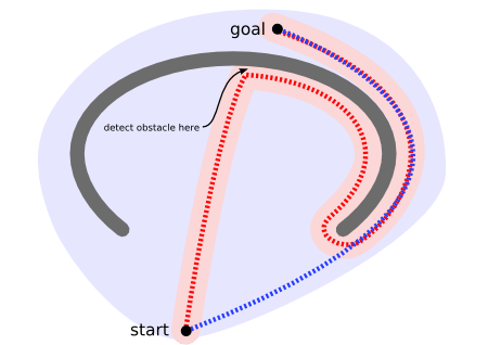
 A non-efficient way to find a path [1]
On a map with many obstacles, pathfinding from points \(A\) to \(B\) can be difficult. A robot, for instance, without getting much other direction, will continue until it encounters an obstacle, as in the path-finding example to the left below.
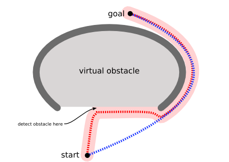
However, the A* algorithm introduces a heuristic into a regular graph-searching algorithm, essentially planning ahead at each step so a more optimal decision is made. With A*, a robot would instead find a path in a way similar to the diagram on the right below.
A* is an extension of Dijkstra's algorithm with some characteristics of breadth-first search (BFS).
 An example of using A* algorithm to find a path [2]
The A* Algorithm
Like Dijkstra, A* works by making a lowest-cost path tree from the start node to the target node. What makes A* different and better for many searches is that for each node, A* uses a function \(f(n)\) that gives an estimate of the total cost of a path using that node. Therefore, A* is a heuristic function, which differs from an algorithm in that a heuristic is more of an estimate and is not necessarily provably correct.
A* expands paths that are already less expensive by using this function:
\[ f(n)=g(n)+h(n), \] where
\(f(n)\) = total estimated cost of path through node \(n\)
\(g(n)\) = cost so far to reach node \(n\)
\(h(n)\) = estimated cost from \(n\) to goal. This is the heuristic part of the cost function, so it is like a guess.
 Using the A* algorithm
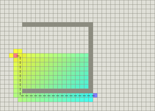
In the grid above, A* algorithm begins at the start (red node), and considers all adjacent cells. Once the list of adjacent cells has been populated, it filters out those which are inaccessible (walls, obstacles, out of bounds). It then picks the cell with the lowest cost, which is the estimated f(n). This process is recursively repeated until the shortest path has been found to the target (blue node). The computation of \(f(n)\) is done via a heuristic that usually gives good results.
The calculation of \(h(n)\) can be done in various ways:
The Manhattan distance (explained below) from node \(n\) to the goal is often used. This is a standard heuristic for a grid.
If \(h(n)\) = 0, A* becomes Dijkstra's algorithm, which is guaranteed to find a shortest path.
The heuristic function must be admissible, which means it can never overestimate the cost to reach the goal. Both the Manhattan distance and \(h(n)\) = 0 are admissible.
Heuristics
Using a good heuristic is important in determining the performance of \(A^{*}\). The value of \(h(n)\) would ideally equal the exact cost of reaching the destination. This is, however, not possible because we do not even know the path. We can, however, choose a method that will give us the exact value some of the time, such as when traveling in a straight line with no obstacles. This will result in a perfect performance of \(A^{*}\) in such a case.
We want to be able to select a function \(h(n)\) that is less than the cost of reaching our goal. This will allow \(h\) to work accurately, if we select a value of \(h\) that is greater, it will lead to a faster but less accurate performance. Thus, it is usually the case that we choose an \(h(n)\) that is less than the real cost.
The Manhattan Distance Heuristic
image
This method of computing \(h(n)\) is called the Manhattan method because it is computed by calculating the total number of squares moved horizontally and vertically to reach the target square from the current square. We ignore diagonal movement and any obstacles that might be in the way.
\[ h = | x_{start} - x_{destination} | + |y_{start} - y_{destination} | \]
This heuristic is exact whenever our path follows a straight lines. That is, \(A^{*}\) will find paths that are combinations of straight line movements. Sometimes we might prefer a path that tends to follow a straight line directly to our destination.
The Euclidean Distance Heuristic
edh
This heuristic is slightly more accurate than its Manhattan counterpart. If we try run both simultaneously on the same maze, the Euclidean path finder favors a path along a straight line. This is more accurate but it is also slower because it has to explore a larger area to find the path.
\[ h = \sqrt{(x_{start} - x_{destination})^2 + (y_{start} - y_{destination})^2 } \]
Can depth-first search always expand at least as many nodes as A* search with an admissible heuristic?
The answer is no, but depth-first search may possibly, sometimes, by fortune, expand fewer nodes than \(A^{*}\) search with an admissible heuristic. E.g.. it is logically possible that sometimes, by good luck, depth-first search may reach directly to the goal with no back-tracking.
The main drawback of the \(A^{*}\) algorithm and indeed of any best-first search is its memory requirement. Since at least the entire open list must be saved, the A* algorithm is severely space-limited in practice, and is no more practical than best-first search algorithm on current machines.
Implementation
The pseudocode for the A* algorithm is presented with Python-like syntax.
1 2 3 4 5 6 7 8 9 10 11 12 13 14 15 16 17 18 | |
The time complexity of \(A^{*}\) depends on the heuristic. In the worst case, the number of nodes expanded is exponential in the length of the solution (the shortest path), but it is polynomial when the search space is a tree.
Examples
Use A* to find the shortest path from the green square to the yellow square in the grid below.

Let us start by choosing an admissible heuristic. For this case, we can use the Manhattan heuristic. We then proceed to the starting cell. We call it our
current celland then we proceed to look at all its neighbors and compute \[f,g,h\] for each of them. We then select the neighbor with the lowest \(f\) cost. This is our newcurrent celland we then repeat the process above.(populate neighbors and compute \(f\),\(g\) and \(h\) and choose the lowest ). We do this until we are at the goal cell. The image below demonstrates how the search proceeds. In each cell the respective \(f\),\(h\) and \(g\) values are shown. Remember \(g\) is the cost that has been accrued in reaching the cell and \(h\) is the Manhattan distance towards the yellow cell while \(f\) is the sum of \(h\) and \(g\).

References
- Patel, A. Introduction to A*. Retrieved April 29, 2016, from http://theory.stanford.edu/~amitp/GameProgramming/concave1.png
- Patel, A. Introduction to A*. Retrieved April 29, 2016, from http://theory.stanford.edu/~amitp/GameProgramming/concave2.png