Conditional Probability Distribution

Conditional probability is the probability of one thing being true given that another thing is true, and is the key concept in Bayes' theorem. This is distinct from joint probability, which is the probability that both things are true without knowing that one of them must be true.

For example, one joint probability is "the probability that your left and right socks are both black," whereas a conditional probability is "the probability that your left sock is black if you know that your right sock is black," since adding information alters probability. This can be high or low depending on how frequently your socks are paired correctly. An Euler diagram, in which area is proportional to probability, can demonstrate this difference.

Let $X$ be the probability that your left sock is black, and let $Y$ be the probability that your right sock is black. On the left side of the diagram, the yellow area represents the probability that both of your socks are black. This is the joint probability $P(X,Y)$. If $Y$ is definitely true (e.g., given that your right sock is definitely black), then the space of everything not $Y$ is dropped and everything in $Y$ is rescaled to the size of the original space. The rescaled yellow area is now the conditional probability of $X$ given $Y$, expressed as $P(X \mid Y)$. In other words, this is the probability that your left sock is black if you know that your right sock is black. Note that the conditional probability of $X$ given $Y$ is not in general equal to the conditional probability of $Y$ given $X$. That would be the fraction of $X$ that is yellow, which in this picture is slightly smaller than the fraction of $Y$ that is yellow.

Philosophically, all probabilities are conditional probabilities. In the Euler diagram, $X$ and $Y$ are conditional on the box that they are in, in the same way that $X | Y$ is conditional on the box $Y$ that it is in. Treating probabilities in this way makes chaining together different types of reasoning using Bayes' theorem easier, allowing for the combination of uncertainties about outcomes ("given that the coin is fair, how likely am I to get a head") with uncertainties about hypotheses ("given that Frank gave me this coin, how likely is it to be fair?"). Historically, conditional probability has often been misinterpreted, giving rise to the famous Monty Hall problem and Bayesian mistakes in science.

For discrete random variables, the conditional probability mass function of $Y$ given the occurrence of the value $x$ of $X$ can be written according to its definition as

$$P(Y = y \mid X = x) = \dfrac{P(X=x \cap Y=y)}{P(X=x)}.$$

Dividing by $P(X=x)$ rescales the joint probability to the conditional probability, as in the diagram in the introduction. Since $P(X=x)$ is in the denominator, this is defined only for non-zero (hence strictly positive) $P(X=x)$. Furthermore, since $P(X = x) \leq 1$, it must be true that $P(Y = y \mid X = x) \geq P(X=x \cap Y=y)$, and that they are only equal in the case where $P(X = x) = 1$. In any other case, it is more likely that $X = x$ and $Y = y$ if it is already known that $X = x$ than if that is not known.

The relation with the probability distribution of $X$ given $Y$ is

$$P(Y=y \mid X=x) P(X=x) = P(X=x\ \cap Y=y) = P(X=x \mid Y=y)P(Y=y).$$

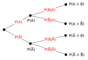
As a concrete example, the picture below shows a probability tree, breaking down the conditional distribution over the binary random variables $A$ and $B$. The four nodes on the right-hand side are the four possible events in the space. The leftmost node has value one. The intermediate nodes each have a value equal to the sum of their children. The edge values are the nodes to their right divided by the nodes to their left. This reflects the idea that all probabilities are conditional. $P(A)$ and $P(B)$ are conditional on the assumptions of the whole probability space, which may be something like "$A$ and $B$ are the outcomes of flipping fair coins."

Similarly, for continuous random variables, the conditional probability density function of $Y$ given the occurrence of the value $x$ of $X$ can be written as

$$f_Y(y \mid X=x) = \dfrac{f_{X, Y}(x, y)}{f_X(x)},$$

where $f_{X, Y} (x, y)$ gives the joint density of $X$ and $Y$, while $f_X(x)$ gives the marginal density for $X$. Also in this case it is necessary that $f_{X} (x) > 0$. The relation with the probability distribution of $X$ given $Y$ is given by

$$f_Y(y \mid X=x)f_X(x) = f_{X,Y}(x, y) = f_X(x \mid Y=y)f_Y(y).$$

The concept of the conditional distribution of a continuous random variable is not as intuitive as it might seem: Borel's paradox shows that conditional probability density functions need not be invariant under coordinate transformations.

Conditional distributions and marginal distributions are related using Bayes' theorem, which is a simple consequence of the definition of conditional distributions in terms of joint distributions.

Bayes' theorem for discrete distributions states that

$$\begin{aligned} P(Y=y \mid X=x) P(X=x) &= P(X=x\ \cap Y=y) \\ &= P(X=x \mid Y=y)P(Y=y)\\\\ \Rightarrow P(Y=y \mid X=x) &= \dfrac{P(X=x \mid Y=y)}{P(X=x)} P(Y=y). \end{aligned}$$

This can be interpreted as a rule for turning the marginal distribution $P(Y=y)$ into the conditional distribution $P(Y=y \mid X=x)$ by multiplying by the ratio $\frac{P(X=x \mid Y=y)}{P(X=x)}$. These functions are called the prior distribution, posterior distribution, and likelihood ratio, respectively.

For continuous distributions, a similar formula holds relating conditional densities to marginal densities:

$$f_{Y} (y \mid X = x) = \dfrac{f_{X}(x \mid Y = y)}{f_{X} (x)} f_{Y} (y).$$

Two variables are independent if knowing the value of one gives no information about the other. More precisely, random variables $X$ and $Y$ are independent if and only if the conditional distribution of $Y$ given $X$ is, for all possible realizations of $X,$ equal to the unconditional distribution of $Y$. For discrete random variables this means $P(Y = y | X = x) = P(Y = y)$ for all relevant $x$ and $y$. For continuous random variables $X$ and $Y$, having a joint density function, it means $f_Y(y | X=x) = f_Y(y)$ for all relevant $x$ and $y$.

Seen as a function of $y$ for given $x$, $P(Y = y | X = x)$ is a probability, so the sum over all $y$ (or integral if it is a conditional probability density) is 1. Seen as a function of $x$ for given $y$, it is a likelihood function, so that the sum over all $x$ need not be 1.

Let $(\Omega, \mathcal{F}, P)$ be a probability space, $\mathcal{G} \subseteq \mathcal{F}$ a $\sigma$-field in $\mathcal{F}$, and $X : \Omega \to \mathbb{R}$ a real-valued random variable $\big($measurable with respect to the Borel $\sigma$-field $\mathcal{R}^1$ on $\mathbb{R}\big).$ It can be shown that there exists a function $\mu : \mathcal{R}^1 \times \Omega \to \mathbb{R}$ such that $\mu(\cdot, \omega)$ is a probability measure on $\mathcal{R}^1$ for each $\omega \in \Omega$ (i.e., it is regular) and $\mu(H, \cdot) = P(X \in H | \mathcal{G})$ (almost surely) for every $H \in \mathcal{R}^1$. For any $\omega \in \Omega$, the function $\mu(\cdot, \omega) : \mathcal{R}^1 \to \mathbb{R}$ is called a conditional probability distribution of $X$ given $\mathcal{G}$. In this case,

$$E[X | \mathcal{G}] = \int_{-\infty}^\infty x \, \mu(d x, \cdot)$$

almost surely.

For any event $A \in \mathcal{A} \supseteq \mathcal B$, define the indicator function

$$\mathbf{1}_A (\omega) = \begin{cases} 1 \; &\text{if } \omega \in A \\ 0 \; &\text{if } \omega \notin A, \end{cases}$$

which is a random variable. Note that the expectation of this random variable is equal to the probability of $A$ itself:

$$\operatorname{E}(\mathbf{1}_A) = \operatorname{P}(A).$$

Then the conditional probability given $\mathcal B$ is a function $\operatorname{P}(\cdot|\mathcal{B}):\mathcal{A} \times \Omega \to (0,1)$ such that $\operatorname{P}(A|\mathcal{B})$ is the conditional expectation of the indicator function for $A$:

$$\operatorname{P}(A|\mathcal{B}) = \operatorname{E}(\mathbf{1}_A|\mathcal{B}).$$

In other words, $\operatorname{P}(A|\mathcal{B})$ is a $\mathcal B$-measurable function satisfying

$$\int_B \operatorname{P}(A|\mathcal{B}) (\omega) \, \operatorname{d} \operatorname{P}(\omega) = \operatorname{P} (A \cap B) \quad \text{for all} \quad A \in \mathcal{A}, B \in \mathcal{B}.$$

A conditional probability is regular if $\operatorname{P}(\cdot|\mathcal{B})(\omega)$ is also a probability measure for all $\omega ∈ \Omega$. An expectation of a random variable with respect to a regular conditional probability is equal to its conditional expectation.

• For a trivial sigma algebra $\mathcal B= \{\emptyset,\Omega\}$ the conditional probability is a constant function, $\operatorname{P}\!\left( A| \{\emptyset,\Omega\} \right) \equiv\operatorname{P}(A)$.

• For $A\in \mathcal{B}$, as outlined above, $\operatorname{P}(A|\mathcal{B})=1_A.$