This wiki is incomplete.

\[\SI{37}{\celsius}\]

\[37\hspace{0.6mm}^{\circ}\hspace{-0.2mm}\text{C}\]

\[\begin{array} x+y \\ -(s+t)

\end{array}

\begin{array} 2x+3y \\ -(4s+3t) \end{array}\]

The two equations are \(2s + t = 5\) and \(s + t = 3.\)

If we subtract the second from the first, we get

\[\begin{align} (2s + t) - (s + t) &= 5 - 3 \\ 2s - s + t - t &= 2 \\ s &= 2 \end{align}\]

Hello this is my x and this is your \(x\)

\(2\pi/\left(\frac{m}{n}\right)\)

\(2\pi/\left(m/n\right)\)

\(\dfrac{2\pi}{\frac{m}{n}}\)

\(\text{8:11 pm}\) \(\text{8:11 PM}\)

Mixed parenthesis

The principles of quantum mechanics (which didn't take shape until the \(1930\)s) recast the laws of nature in ways that still aren't fully understood. Part of the core of these new ideas is the principle of superposition, that the state of a particle can consist of two mutually exclusive observable states \(\ket{\psi} = \frac{1}{\sqrt{2}}\left(\ket{-} + \ket{+}\right)\).

Furthermore, particles can be entangled, so that the state of two particles can't be separated to those of individual particles: \[{\ket{\psi}_{AB} \neq \left(c_1\ket{-} + c_2\ket{+}\right)\otimes\left(c_3\ket{-} + c_4\ket{+}\right)}.\]

Currently, it isn't fully understood how these principles conspire to produce various quantum phenomena (for example, the jury is still out on how much of the speedup in quantum computing can be attributed to entanglement).

TeX parenthesis only

The principles of quantum mechanics \((\)which didn't take shape until the \(1930\)s\()\) recast the laws of nature in ways that still aren't fully understood. Part of the core of these new ideas is the principle of superposition, that the state of a particle can consist of two mutually exclusive observable states \(\ket{\psi} = \frac{1}{\sqrt{2}}\left(\ket{-} + \ket{+}\right)\).

Furthermore, particles can be entangled, so that the state of two particles can't be separated to those of individual particles: \[{\ket{\psi}_{AB} \neq \left(c_1\ket{-} + c_2\ket{+}\right)\otimes\left(c_3\ket{-} + c_4\ket{+}\right)}.\] Currently, it isn't fully understood how these principles conspire to produce various quantum phenomena \((\)for example, the jury is still out on how much of the speedup in quantum computing can be attributed to entanglement\()\).

\[{\pmb a}\]

\[\frac{(-4)^3}{(-7)^3}\] \[\dfrac{(-4)^3}{(-7)^3}\] \[(-4)^3/(-7)^3\]

there are \(\numcomma{13000}\) cookies in my desk.

\(\square\,\pmb{\square}\)

the total entropy never decreases: \(\Delta S_\text{total} \geq 0.\)

putting this in terms of a system and its surroundings...

\[\Delta S_\text{surr} + \Delta S_\text{sys} \geq 0\]

the entropy change in the surrounding is the heat flow from the system, over temperature

\[-\frac{Q}{T} + \Delta S_\text{sys} \geq 0\]

but the heat flow into the system is the work the system did plus its rise in internal energy: \(Q = \Delta E + W.\) work can be mechanical (\(P\cdot dV\)) or non-mechanical, so \(W = W_\text{mech} + W_\text{not mech}.\)

putting this altogether, we get

\[-\frac{\Delta E + P\Delta V + W_\text{not mech}}{T} + \Delta S_\text{sys} \geq 0\]

or

\[ \boxed{0 \geq \Delta E + P\Delta V + W_\text{not mech} - T\Delta S_\text{sys}} \]

when no mechanical work is done at all (mechanical or otherwise), this is

\[-W_\text{not mech} \leq \Delta E - T\Delta S_\text{sys} = \Delta F\]

when volume varies, the right side would be the change in \(G\) so long as pressure and temperature are held constant (\(G = E - TS + PV\) so \(\Delta G = \Delta E - T\Delta S - S\Delta T + P\Delta V + V\Delta P\) and \(\Delta G = \Delta E + P\Delta V - T\Delta S\) when pressure and temperature are maintained).

if you want to look at enthalpy (\(H = E + PV\)), the above shows it's always less than negative the change in entropy, and has its own minimal principle if you can somehow maintain entropy.

When evaluating the likelihood of various explanations in light of a stream of information, the assessment up to the current moment can be held in memory and updated on the fly when each new piece of evidence comes online. Suppose we want to infer Israeli intentions toward Syria. One hypothesis \(\mathcal{H_1}\) might be “Israel is planning to launch a major offensive against Syria within 30 days” and the other \(\mathcal{H_2}\) might be, “Israel is not planning to launch a major offensive against Syria within 30 days”.

If we consider the two competing hypotheses to be the only possible underlying explanations for the unfolding of events relevant to Israel-Syria relations, we can visualize the problem as a two layered graph with edges between \(\mathcal{H_1}\) and all the evidence nodes \(E_1, \ldots, E_n\) (which can be collected as \(\vec{E_n}\)) and between the evidence nodes and \(\mathcal{H_2}\), but not between the two hypothesis nodes or between any pair of evidence nodes.

To start, let’s assign a number to our prior belief about our hypotheses. For the sake of argument, suppose we have little confidence in the belief that Israel plans to imminently attack Syria, so we put this belief at 5%. Thus: \[p(\mathcal{H_1}=\mbox{attack plan}) = 5\%\] and \[p(\mathcal{H_2} = \mbox{no attack plan}) = 95\%\]Now suppose we find out that the finance minister in Israeli makes a public statement to the effect “the nation’s economic situation is one of war and scarcity, not one of peace and prosperity.” This is the first piece of evidence \(E_1\). We ask, how likely is it that such a statement would be made if Israel was planning for war? Or: what is \(p(E_1=\mbox{Finance minister statement}|\mathcal{H_1} = \mbox{attack plan})\)?

We are not very confident that the finance minister would say this if Israel had war plans because it would give away the element of surprise, we assign \(p(E_1|\mathcal{H_1})=50\%\). We have more belief that this statement would be made given no war plans, to benefit from any deterrence it might ingrain, thus \(p(E_1|\mathcal{H_2})=85\%\).

Now, we compute the belief in \(\mathcal{H_1}\) light of the statement, \(E_1\). The conditional belief \(p(\mathcal{H1}|E_1)\) is equal to the joint belief \(p(\mathcal{H_1},E_1)\) normalized to the total chance of the statement \(p(E_1)\). \[p(\mathcal{H_1}|E_1)=\frac{p(\mathcal{H_1},E_1)}{p(E_1)}=\frac{p(E_1|\mathcal{H_1})\times p(H_1)}{\sum\limits_i p(E_1|\mathcal{H_i})\times p(\mathcal{H_i})}=\frac{0.5\times0.05}{0.5\times0.05+0.85\times0.95}=3\%\]

Prior to receiving any information about the finance minister’s statement, we held a weak 5% belief in their being an Israeli plan to attack Syria within the next thirty days. In light of his statement regarding the economic situation, our belief has fallen to just 3%. We would like to accumulate wisdom as we go along and to be able to incorporate new information in a simple manner. Suppose we have already incorporated \(n\) pieces of evidence \(E_n\) so that our belief in the first hypothesis is given by \[p(\mathcal{H_1}|E_1,\ldots,E_n) \sim p(E_1,\ldots,E_n|\mathcal{H_1})\times p(\mathcal{H_1})\] or \[p(\mathcal{H_1}|\vec{E_n})\sim p(\vec{E_n}|\mathcal{H_1})\times p(\mathcal{H_1})\]We receive a new bit of evidence \(E_{n+1}\) so that our belief in the hypothesis becomes \[p(\mathcal{H_1}|\vec{E_{n+1}})\sim p(E_1,\ldots,E_n,E_{n+1}|\mathcal{H_1})\times p(\mathcal{H_1})\] We can rewrite the first term on the right side by conditioning \(E_{n+1}\) on \(E_1\) through \(E_n\) so that we recover the expression for \(n\) items of evidence as a factor: \[p(\mathcal{H_1}|\vec{E_{n+1}})\sim p(E_{n+1}|E_1,\ldots,E_n,\mathcal{H_1})\times p(E_1,\ldots,E_n|\mathcal{H_1})\times p(\mathcal{H_1})\] Since each piece of evidence in the stream is assumed to be independent of the other evidence, we can write \(p(E_{n+1}|\vec{E_n},\mathcal{H1}) \sim p(E_{n+1}|\mathcal{H_1})\).

Therefore, we have the simple update rule \[p(\mathcal{H_1}|\vec{E_{n+1}}) \sim p(E_{n+1}|\mathcal{H_1})\times p(\vec{E_n}|\mathcal{H_1})p(\mathcal{H_1})\]

Finally, this becomes \[p(\mathcal{H_1}|\vec{E_{n+1}})\sim p(E_{n+1}|\mathcal{H_1})\times p(\mathcal{H_1}|\vec{E_n})\] an easy to work with, recursive update rule. Very simply, each time we receive a new piece of evidence, we ask how strong our belief is for this evidence to have been produced under the hypothesis in question.

This is commonly expressed as \(R = L \times P\) with \(R\) the revised estimate for the hypothesis, \(L\) the likelihood of the new evidence given the hypothesis, and \(P\) the prior belief for the hypothesis. Each new piece of evidence in the stream introduces another \(L\) to modify the belief. Clearly, after each update, we normalize so that the sum over all the hypotheses, given the stream of evidence, is 1. In this way, we can easily incorporate new evidence into our belief in competing underlying explanations.

For sake of argument, we learn that Israel has mobilized the 7th brigade to the Syrian border and call this the second piece of evidence, \(E_2\). We have very little belief that this would occur if Israel did not have plans to engage Syria, and so, \(p(E_2|\mathcal{H_2})=1\%\). We believe there is a high chance Israel would do this given plans for invasion, thus \(p(E_2|\mathcal{H_1})=70\%\). Our current beliefs in the two hypotheses are \(p(\mathcal{H_1}|E_1) = 3\%\) and \(p(\mathcal{H_2}|E_1)=97\%\). Our update yields \[p(\mathcal{H_1}|E_1,E_2) \sim p(E_2|\mathcal{H_1})\times p(\mathcal{H_1}|E_1)=70\%\times3\%\] and \[p(\mathcal{H_2}|E_1,E_2) \sim p(E_2|\mathcal{H_2})\times p(\mathcal{H_2}|E_1)=1\%\times97\%\] Normalizing, we find that our belief in \(\mathcal{H_1}\) (the belief that Israel is preparing for military action against Syria) has risen significantly to \(68\%\) given the new evidence in the border activity while our belief in \(\mathcal{H_2}\) has fallen to just \(32\%\).

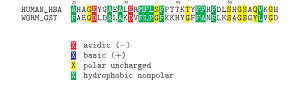
This pair of alleles is \(AaBbCC\) or \(\text{AaBbCC}\) or \(\textbf{AaBbCC}\) or \(\tt{AaBbCC}\) or AaBbCC or AaBbCC

This is my paragraph about numbers This is my paragraph about numbers This is my paragraph about numbers This is my paragraph about numbers This is my paragraph about numbers This is my paragraph about numbers This is my paragraph about numbers This is my paragraph about numbers \(\frac38.\) This is my paragraph about numbers This is my paragraph about numbers This is my paragraph about numbers This is my paragraph about numbers This is my paragraph about numbers This is my paragraph about numbers.

This is my paragraph about numbers This is my paragraph about numbers This is my paragraph about numbers This is my paragraph about numbers This is my paragraph about numbers This is my paragraph about numbers This is my paragraph about numbers This is my paragraph about numbers \(\dfrac38.\) This is my paragraph about numbers This is my paragraph about numbers This is my paragraph about numbers This is my paragraph about numbers This is my paragraph about numbers This is my paragraph about numbers.

An example of a transformation that's not linear is \(T(\mathbf{x}) = \mathbf{x}\cdot\mathbf{x},\) since \((\mathbf{a} + \mathbf{b})\cdot(\mathbf{a} + \mathbf{b}) \neq a^2 + b^2\) in general. So, transformations where the arguments being multiplied together are non-linear transformations.

Now take a look at the transformation \(T(\mathbf{x}) = \mathbf{x} + \mathbf{k}\) where \(\mathbf{k}\) is some fixed vector. As a specific example, suppose \(\mathbf{x} = \begin{pmatrix} -2 & 1 & 5 \end{pmatrix}^\text{T}\) and \(\mathbf{k} = \begin{pmatrix} 7 & 3 & 3 \end{pmatrix}^\text{T}\). The action of the transformation is then

\[T(\mathbf{x}) = \begin{pmatrix} -2 \\ 1 \\ 5 \end{pmatrix} + \begin{pmatrix} 7 \\ 3 \\ 3 \end{pmatrix} = \begin{pmatrix} 5 \\ 4 \\ 8 \end{pmatrix}.\]

Is \(T\) a linear transformation?

This is my paragraph about all my favorite things like Vaporeon, Sylveon, Glaceon, Jolteon, and Flareon. I am also passionate about functions like \(f(x)= x^2\) as well as functions like \(\frac{x}{\sqrt{1+x^2}}.\) Notice that when \(x\) is small, the function is nearly linear. I also have other thresholding functions that I like to talk about like \(\frac{x}{1+x}\) and \(\frac{1}{1+e^{-x}}.\) All of these can be used to model a neuron, if you like.

This is my paragraph about all my favorite things like Vaporeon, Sylveon, Glaceon, Jolteon, and Flareon. I am also passionate about functions like \(f(x)= x^2\) as well as functions like \(x/\sqrt{1+x^2}.\) Notice that when \(x\) is small, the function is nearly linear. I also have other thresholding functions that I like to talk about like \(x/(1+x)\) and \(1/(1+e^{-x}).\) All of these can be used to model a neuron, if you like. Derivatives I like include \(dy/dx\) and \(\frac{dx}{dt}.\)

This is my paragraph about all my favorite things like Vaporeon, Sylveon, Glaceon, Jolteon, and Flareon. I am also passionate about functions like \(f(x)= \lim_{\epsilon\rightarrow 0}x^{2+\epsilon}\) or \(f(x)= \lim\limits_{\epsilon\rightarrow 0}x^{2+\epsilon}\) as well as functions like \[\frac{x}{\sqrt{1+x^2}}.\] Notice that when \(x\) is small, the function is nearly linear. I also have other thresholding functions that I like to talk about like \[\frac{x}{1+x}\] and \[\frac{1}{1+e^{-x}}.\] All of these can be used to model a neuron, if you like.

\[\SI[per-mode=symbol]{5}{\meter\per\second\squared}\]

In the year 1890, Sherlock Holmes lived at 47 Main St. He brought 15 orbs in a velvet satchel. The chance of rain was 23%. In the year 1890, Sherlock Holmes lived at 47 Main St. He brought 15 orbs in a velvet satchel. The chance of rain was 23%.

In the year 1890, Sherlock Holmes lived at 47 Main St. He brought \(15\) orbs in a velvet satchel. The chance of rain was \(23%.\) In the year 1890, Sherlock Holmes lived at 47 Main St. He brought \(15\) orbs in a velvet satchel. The chance of rain was \(23%.\)

In the year \(1890,\) Sherlock Holmes lived at \(47\) Main St. He brought \(15\) orbs in a velvet satchel. The chance of rain was \(23%.\) In the year \(1890,\) Sherlock Holmes lived at \(47\) Main St. He brought \(15\) orbs in a velvet satchel. The chance of rain was \(23%.\)

YES \[\frac{4}{3}x^{4/3} \] NO \[x^{\frac{4}{3}}\]

\[ \dfrac{1 + {\color{E1503C}\sqrt{\text{top}}}}{1 - {\color{2C6FEF}\sqrt{\text{bottom}}}} + {\color{EEA71F}\mathbf{H}\cdot\mathbf{H}} \]

This is Big \(O\) notation. The runtime of merge-sort is \(O(n\log n).\)

This is Big-\(O\) notation. The runtime of merge-sort is \(O(n\log n).\)

This is Big O notation. The runtime of merge-sort is \(O(n\log n).\)

This is big \(O\) notation. The runtime of merge-sort is \(O(n\log n).\)

This is Big-O notation. The runtime of merge-sort is \(O(n\log n).\)

Let's take care of the square inside the expectation first:

\[ (X_{i}-\bar{X})^2 = X_{i}^2 - 2 X_{i} \bar{X} + \bar{X}^2,\]

so when we sum, we find

\[ \sum\limits_{i=1}^{n} (X_{i} - \bar{X} )^2 = \sum\limits_{i=1}^{n} X_{i}^2 - 2 n \bar{X}^2 + n \bar{X}^2 = \sum\limits_{i=1}^{n} X_{i}^2 - n \bar{X}^2.\]

Here, we used the definition \( n \bar{X} = \sum_{i=1}^{n} X_{i}.\)

By the linearity of expectation,

\[ E \left[ \sum\limits_{i=1}^{n} (X_{i} - \bar{X} )^2 \right] = \sum\limits_{i=1}^{n} E[X_{i}^2] - n E[\bar{X}^2].\]

Each of the random variables has variance \( \sigma^2,\) which implies

\[ E[(X_{i} - \mu)^2] = E[X_{i}^2] - \mu^2 = \sigma^{2}, \]

so

\[ \sum\limits_{i=1}^{n} E[X_{i}^2] = n (\sigma^2 + \mu^2)\]

and

\[ E \left[ \sum\limits_{i=1}^{n} (X_{i} - \bar{X} )^2 \right] = n (\sigma^2 + \mu^2 - E[\bar{X}^2]).\]

As tempting as it would be to say that \( E[\bar{X}^2] = \mu^2\) in order to have the last two terms cancel, this is false. Special care is needed in order to handle \( \mu^2 - E[\bar{X}^2]).\)

By definition, \( \bar{X} = \frac{1}{n} \sum_{i=1}^{n} X_{i},\) and so

\[ \begin{align} \bar{X}^2 & = \frac{1}{n^2} \left(\sum_{i=1}^{n} X_{i}\right)^2 \\ & = \frac{1}{n^2} \sum_{i=1}^{n} X_{i} \times \sum_{i=j}^{n} X_{j} \\ & = \frac{1}{n^2} \sum\limits_{i,j=1}^{n} X_{i} X_{j}. \end{align}.\]

We introduced another dummy index in the sum over the random variables in order to get the product of \( \bar{X}\) with itself right.

(If this step isn't clear, pick your favorite value of \(n\) and square \( \bar{X}\) explicitly to see what the terms look like.)

We split the sum above as follows:

\[ \frac{1}{n^2} \sum\limits_{i,j=1}^{n} X_{i} X_{j} = \frac{1}{n^2} \sum\limits_{i=1}^{n} X_{i}^2 + \frac{1}{n^2} \sum\limits_{i,j=1, i \neq j}^{n} X_{i} X_{j}.\]

Taking the expectation of both sides gives us

\[ E[\bar{X}^2] = \frac{1}{n^2} \times n \times ( \mu^2 + \sigma^2) + \frac{1}{n^2} \sum\limits_{i,j=1, i \neq j}^{n} \mu^2;\]

remember, the \(X_{i}\)'s are independent random variables, so

\[ E[X_{i} X_{j} ] = E[X_{i}] E[X_{j}] = \mu \times \mu = \mu^2\]

when \( i \neq j.\)

Since there are \(n(n-1)\) terms in the sum

\[ \sum\limits_{i,j=1, i \neq j}^{n} \mu^2\]

and they're all equal to \( \mu^2, \) we arrive at the result:

\[ \begin{align} E[\bar{X}^2] & = \frac{1}{n} \left( \mu^2 + \sigma^2 \right)+ \frac{n(n-1)}{n^2} \mu^2 \\ & = \mu^2 + \frac{1}{n} \sigma^2. \end{align} \]

In conclusion,

\[ \begin{align} E \left[ \sum\limits_{i=1}^{n} (X_{i} - \bar{X} )^2 \right] & = n (\sigma^2 + \mu^2 - E[\bar{X}^2]) \\ & = n ( \sigma^2 - \frac{1}{n} \sigma^2) \\& = (n-1) \sigma^2, \end{align} \]

and \( c = n-1.\)

Consider the \(E\)-component of an electromagnetic wave in a lasing cavity of length \(\ell.\) The waves are generated by a current \(J(x)\) that permeates the cavity and the walls are made by a perfectly reflective, conducting material, so \(E_z(0)=E_z(L)=0.\) Maxwell's equation for the \(E\)-component (polarized in the \(z\) direction) is \[\left(\frac{\partial^2}{\partial x^2} - k^2\right)E_z(x) = J(x)\]

where the constant \(k\) is equal to \(\frac{g\omega^2}{c^2}\) where \(c\) is the speed of light, \(\omega\) is the angular frequency of the light, and \(g\) is the gain coefficient, a number that describes the transfer of energy from the medium to the electromagnetic wave.

Find the general solution for \(E_z\) between the walls.

The big idea of Green's approach is that the entire current \(J(x)\) is contributing to the solution for the field and that we can split it up into little packets of current, represented by delta functions at all points \(y\) between the walls. If we can find the contribution to the field at \(x\) from one of these little packets at \(y,\) \(G(x,y)\), then we can just add them up to get the overall field: \(E_z(x) = \int dy\, G(x,y)J(y).\)

So, we start with

\[\dfrac{\partial^2}{\partial x^2}G(x,y) - k^2G(x,y) = \delta(x-y)\]

The \(\delta\)-function at \(y\) is a nasty bump that's going to cause the solution to have a discontinuous derivative as mentioned above. Just to see for ourselves, we can integrate this equation across \(y.\)

\[\begin{align} \int_{y-\varepsilon}^{y+\varepsilon} dx\, \dfrac{\partial^2G}{\partial x^2} &= \int_{y-\varepsilon}^{y+\varepsilon} dx\, \delta(x-y) + \int_{y-\varepsilon}^{y+\varepsilon} dx\, k^2 G \\ \dfrac{\partial G}{\partial x}\bigg|_{x=y+\varepsilon} - \dfrac{\partial G}{\partial x}\bigg|_{x=y-\varepsilon} &= 1 + k^2 \int_{y-\varepsilon}^{y+\varepsilon} dx\, G \end{align}\]

In the limit where \(\varepsilon\) goes to \(0,\) the integral on the right becomes zero since the integral of a continuous function over zero range is zero (\(G\) is not itself a \(\delta\)-function), and we're left with the promised unit jump in the value of the derivative at \(x=y.\) Only the second order term will contribute on the left hand side in this integral since everything else will be the integral of a continuous function with no range, so it becomes

\[\frac{\partial G}{\partial x}\bigg|_{x=y+\varepsilon} = 1 + \frac{\partial G}{\partial x}\bigg|_{x=y-\varepsilon}\]

Because of the jump discontinuity in the derivative of \(G,\) we expect distinct solutions on either side of \(x = y,\) where the \(\delta\)-function is \(0.\) The general solution of \(\partial_x^2G(x,y) - k^2G(x,y) = 0\) is \[A(y)e^{kx} + B(y)e^{-kx}.\] In particular, we'll write the left- and right-hand solutions like \[\begin{align} G_L(x,y) &= L_1(y)e^{kx} + L_2(y)e^{-kx} \\ G_R(x,y) &= R_1(y)e^{kx} + R_2(y)e^{-kx} \end{align}\]

Because the walls are reflective conductors, the field has to be zero at them: \(G(0,y) = G(\ell,y) = 0.\) This leads us to \(L_1(y) = -L_2(y)\) and \(R_2(y) = -e^{2k\ell}R_1(y).\)

This leads us to

\[\begin{align} G_L(x,y) &= L^\prime_1(y)\sinh{kx} \\ G_R(x,y) &= R_1(y)\left(e^{kx} - e^{2k\ell}e^{-kx}\right) \\ &= R_1^\prime(y)\sinh{k(x-\ell)} \end{align}\]

where we have pulled a factor of \(2e^{-kl}\) into \(R_1(y)\) and a factor of \(2\) into \(L_1(y).\) This still has two unknown coefficients \(L^\prime_1(y)\) and \(R^\prime_1(y).\) To find those, we have two more constraints that we can exploit:

The solution has to be unique at \(x=y\) so \(G_L(y,y) = G_R(y,y).\)
The derivative jumps by \(1\) at \(x=y,\) as we showed above.

In terms of the solutions, these constraints are:

\[\begin{align} L^\prime_1(y)\sinh{y} &= R_1^\prime(y)\sinh{k(y-\ell)} \\ kR_1^\prime(y)\cosh{k(y-\ell)} &= 1 + kL^\prime_1(y)\cosh{ky}. \end{align}\]

Solving the two equations leads to

\[\begin{align} L^\prime_1(y) &= \frac{1}{k}\dfrac{\sinh{k(y-\ell)}}{\sinh{k\ell}} \\ R^\prime_1(y) &= \frac{1}{k}\dfrac{\sinh{ky}}{\sinh{k\ell}}, \end{align}\]

so that

\[\begin{align} G_L(x,y) &= \frac{1}{k}\dfrac{\sinh{k(y-\ell)}}{\sinh{k\ell}}\sinh{kx} \\ G_R(x,y) &= \frac{1}{k}\dfrac{\sinh{ky}}{\sinh{k\ell}}\sinh{k(x-\ell)} \end{align}\]

Now, all we have to do is integrate the Green's function against the current function \(J:\) \[\begin{align} E_z(x) &= \int\limits_0^{\ell} dy\, G(x,y)J(y) \\ &= \int\limits_0^{x} dy\, G_R(x,y)J(y) + \int\limits_x^{\ell} dy\, G_L(x,y)J(y) \\ &= \int\limits_0^{x} dy\, \frac{1}{k}\dfrac{\sinh{ky}}{\sinh{k\ell}}\sinh{k(x-\ell)}J(y) + \int\limits_x^{\ell} dy\, \frac{1}{k}\dfrac{\sinh{k(y-\ell)}}{\sinh{k\ell}}\sinh{kx}J(y) \end{align}\]

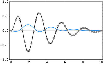
We can test this out on a few trial currents. In the plots below, the \(\color{gray}\text{gray}\) curve represents the current \(J(x),\) the \(\color{blue}\text{blue}\) curve represents the resulting field, and the \(\color{black}\text{black}\) points represent the expression \(\left(\frac{\partial^2}{\partial x^2} - k^2\right)G(x,y)\) which we expect to be equal to \(J(x).\)

In the first example, \(J(x) = xe^{-5x/\ell}\sin\frac{25 x}{\ell}\cos\frac{x}{\ell}\) and \(k=0.02:\)

In the second example, we use \(J(x) = \left(\ell - x\right)e^{-x^2/\ell^2}\) and \(k=0.6:\)

\[\begin{align} G_{4\rightarrow 1}(z) &= \frac{1}{1-P_{4\rightarrow 4}z}\left(P_{4\rightarrow 1} z + P_{4\rightarrow 2\text{B}} z G_{2\text{B}\rightarrow 1} + P_{4\rightarrow 2\text{I}} z G_{2\text{I}\rightarrow 1} + P_{4\rightarrow 3} \cdot z\cdot \frac{1}{1-P_{3\rightarrow 3}\cdot z}\left(P_{3\rightarrow2\text{I}} \cdot z G_{2\text{I}\rightarrow 1} + P_{3\rightarrow2\text{B}} \cdot z \cdot G_{2\text{B}\rightarrow 1} + P_{3\rightarrow 1}\cdot z\right)\right) \\ G_{2I\rightarrow 1} &= P_{2I\rightarrow 1}\cdot z + P_{2I\rightarrow 2B}\cdot z \frac{1}{1-P_{2B\rightarrow 2B}\cdot z}\left(P_{2B\rightarrow 1} \cdot z + z P_{2B\rightarrow 2I} G_{2I\rightarrow 1}\right) \\ G_{2B\rightarrow 1} &= P_{2B\rightarrow 1}\cdot z + P_{2B\rightarrow 2I}\cdot z \frac{1}{1-P_{2I\rightarrow 2I}\cdot z}\left(P_{2I\rightarrow 1} \cdot z + z P_{2I\rightarrow 2B} G_{2B\rightarrow 1}\right) \end{align}\]

Quiz: Indistinguishable Particles

Pane 1 In the last quiz, we showed that quantum systems violate Bell’s inequality. We really have to accept the notion that a system can be in a superposition of different quantum states simultaneously. We saw that this leads to some pretty startling conclusions about the quantum state of the antimuon and neutrino that were created as a result of the charged pion decay. Before measurement, the state was found to be an entangled superposition of all the possible spin configurations compatible with spin conservation. A spin measurement on one of the particles then truly collapsed the state vector and instantaneously affected the spin of the other particle. Quantum superposition leads to some very interesting consequences when we deal with many particle systems where the particles are of the same type. These particles are said to be indistinguishable. We will spend the remainder of the quiz explaining what indistinguishability means in quantum mechanics and some of the things that it implies for the multiparticle states that indistinguishable particles are allowed to be in.

Pane 2

Before going to the quantum world, let’s think about indistinguishability in the macroscopic, classical world. We can talk about identical twins or look at two freshly minted one dollar bills and call them identical. These are examples of things that look, at first glance, to be the same.

But let’s say that you observed the twins from birth. Undeniably, one twin popped out before the other. Let’s put an unerasable mark on the first twin that came out and another different mark on the other twin. Sure, they may look exactly the same but each has a mark that distinguishes one from the other. Now, as their lives continue, you may see that one prefers to go the gym after work every day while the other loves to play video games most of the day and only eats al-pastor super-burritos. The two twins have been marked from birth to be different but also have different preferences and histories. We can certainly distinguish between the two twins.

Now let's imagine a situation where a detonation in the Earth's core is enough to rip the Earth apart into two seemingly identical chunks. Let’s call one of the objects as Half-of-Earth A and the other as Half-of-Earth B. Half Earth of A and B go hurtling apart in different directions as illustrated below.

Question What are some of the things that would help us to distinguish Half-of-Earth A from Half-of-Earth B? (Can choose more than one).

We can distinguish Half-of-Earth A from Half-of-Earth B by tracking their evolution. This can be done by making successive measurements of the position/momenta of the two objects. We can use the position/momentum initial conditions of the two to distinguish between them. Two classical objects cannot share the same position/momenta coordinates at the same time.

Pane 3 It turns out that, in the macroscopic world, I can distinguish between the two "identical" objects by simply measuring the momentum and position of the two objects at some point and tracking their evolution by measurement. That is in effect what we did with the twins. What about the quantum world? Let’s go back to our antimuon and neutrino example. The spin state ket for this system is:

\( \ket{\psi}=\frac{1}{\sqrt{2}}\Big(\ket{\uparrow}_{\mu^+}\ket{\downarrow}_{\nu_\mu}-\ket{\downarrow}_{\mu^+}\ket{\uparrow}_{\nu_\mu}\Big) \)

Imagine for the sake of argument that I now I have two detectors A and B measuring spin that are on opposite sides of a very thin tunnel. The pion is in the center of the tunnel where it decays. Let’s say that the antimuon and the neutrino are constrained in the tunnel and can only travel towards detector A or B.

Both particles have equal amplitudes for going towards either detector and furthermore their amplitudes do not depend in any way on the spin of the particles. For simplicity, assume that the pion was at rest before the decay. Note that the total momentum is conserved.

Question What does this imply for the antimuon and neutrino?

The antimuon flies away with a definite direction to one detector. The neutrino must have equal magnitude and oppositely directed momentum and thus flies away towards the other detector. The antimuon and neutrino are in a superposition of states where either particle has amplitudes for hitting either detector but their momentum must be equal and opposite. The particles can fly in any direction and are not correlated. There is an amplitude for both particles going to detector A.

Pane 4

This looks very similar to the conditions that led us to requiring that the antimuon and neutrino spins be described by an entangled spin state. Just like the constraint that the spins must be anticorrelated as dictated by spin conservation, the momentum of the two particles are anticorrelated by conservation of momentum. Analogous to the case of spins, each particle has simultaneous amplitudes for being in one state or the other -- in this case, going towards detector A and B. Now let’s denote the state representing the muon going to detector A and neutrino going to detector B as ket \( \ket{A}_{\mu^+}\ket{B}_{\nu_\mu} \).

Question:

Which of the following state kets encode the necessary information that the antimuon and neutrino have simultaneous amplitudes for going towards each detector and that their momentum is anti-correlated?

\( \ket{A}_{\mu^+}\ket{B}_{\nu_\mu}\)
\( \frac{1}{2}\Big(\ket{A}_{\mu^+}+\ket{B}_{\mu^+}\Big)\Big(\ket{A}_{\nu_\mu}+\ket{B}_{\nu_\mu}\Big)\)
\( \frac{1}{\sqrt{2}}\Big(\ket{A}_{\mu^+}\ket{B}_{\nu_\mu}+\ket{B}_{\mu^+}\ket{A}_{\nu_\mu}\Big)\)

Pane 5

The full quantum state should describe the spin of the particles and which detector each particle goes towards. Remember that the decay is such that the direction that the antimuon and neutrino are emitted has no dependence on their spin. The two properties are totally independent of each other. We encountered states like this when we were discussing multiparticle spin states where the spin of each particle was independent of all the others. We used the statistical independence of the spins of different particles to deduce that the quantum state representing the joint multiparticle spin state must be a product state formed from the individual single particle spin kets. From the standpoint of statistics and probability, there is no difference between independent spins on different particles and independent properties of a single particle. They are all just physical quantities that are independent of each other.

Question: Using the independent multiparticle spin states as a guide, what could be the full quantum state vector of the antimuon and neutrino?

\( \frac{1}{\sqrt{2}}\Big(\ket{A}_{\mu^+}\ket{B}_{\nu_\mu}+\ket{B}_{\mu^+}\ket{A}_{\nu_\mu}\Big)+\Big(\ket{\uparrow}_{\mu^+}\ket{\downarrow}_{\nu_\mu}\Big) \)
- \( \frac{1}{\sqrt{2}}\Big(\ket{A}_{\mu^+}\ket{B}_{\nu_\mu}+\ket{B}_{\mu^+}\ket{A}_{\nu_\mu}\Big)+\Big(\ket{\uparrow}_{\mu^+}\ket{\downarrow}_{\nu_\mu}-\ket{\downarrow}_{\mu^+}\ket{\uparrow}_{\nu_\mu}\Big) \)
\( \frac{1}{2}\Big(\ket{A}_{\mu^+}\ket{B}_{\nu_\mu}+\ket{B}_{\mu^+}\ket{A}_{\nu_\mu}\Big)\Big(\ket{\uparrow}_{\mu^+}\ket{\downarrow}_{\nu_\mu}-\ket{\downarrow}_{\mu^+}\ket{\uparrow}_{\nu_\mu} \Big) \)

Pane 6 We now have the full entangled state of the antimuon and neutrino before a measurement is made. Now, the antimuon and neutrino are different particles. The antimuon has a charge +e and mass a little over two hundred times the mass of an electron. The neutrino, on the other hand, is charge neutral and is nearly massless.

Question What are some ways that my detector could be made to also distinguish between the antimuon and the neutrino? (Choose more than one) Design the detector so that it measures the spin and the charge of the particle. The detector does not need to be redesigned in anyway. We can use the spin of the particles to distinguish between the two. Design the detector so that it measures the spin and the mass of the particle.

Pane 7

For particles of different types I could design a detector that not only determines the spin but also measures the charge or mass. There are many ways to do this. For example, passing a spin-1/2 particle through a Stern-Gerlach analyzer will split the beam into the two spin components. But if the particle is charged, it will also have a deflection due to the Lorentz force \( \vec{F} = q \vec{v}\times\vec{B} \). The resultant trajectory of the particle will, in general, then depend on its charge and mass as well as its spin. With a little redesign, the detector can then can be used to determine the mass, charge, and spin together. Let’s say that some time after the pion decay, detector A registers a particle with positive charge +e, a mass 200 times that of an electron, and a spin up.

Question What quantum state has this measurement collapsed the two particle state to? \( \frac{1}{\sqrt{2}}\Big(\ket{A}_{\mu^+}\ket{B}_{\nu_\mu}+\ket{B}_{\mu^+}\ket{A}_{\nu_\mu}\Big)\ket{\uparrow}_{\mu^+}\ket{\downarrow}_{\nu_\mu} \) \( (\ket{B}_{\mu^+}\ket{A}_{\nu_\mu}\ket{\uparrow}_{\mu^+}\ket{\downarrow}_{\nu_\mu} \) \( (\ket{A}_{\mu^+}\ket{B}_{\nu_\mu}\ket{\uparrow}_{\mu^+}\ket{\downarrow}_{\nu_\mu} \)

Pane 8 The two particles are distinguishable and the act of measurement has collapsed the entangled state in such a way that right after the measurement I know that the antimuon is at detector A with spin up and the neutrino is at detector B with spin down.

There is no ambiguity of where each particle is after the measurement. The final state vector after measurement then is \( (\ket{A}_{\mu^+}\ket{B}_{\nu_\mu}\ket{\uparrow}_{\mu^+}\ket{\downarrow}_{\nu_\mu} \). Let’s say that I decide to swap the states that the particles are in such that the antimuon is in the quantum state that the neutrino is in and vice-versa. This sort of swap is known as permutation. In this case, \( A \rightarrow B \), \( B \rightarrow A \) and \( \uparrow \rightarrow \downarrow \) and \( \downarrow \rightarrow \uparrow \).

Question Does this permuted state vector correspond to the same physical configuration of the particles? Yes. No

Pane 9 Now, let’s imagine a slightly different situation. Here two neutrons, each spin 1/2, are released from a spin 0 parent atom at rest which is in the process of a nuclear decay. The particular decay is such that each of the emitted neutrons has an amplitude for being emitted in any direction. We have a detector A and a detector B aligned to measure along the same quantization axis and on opposite sides of the parent atom. They are at equal distance from the parent atom. The resultant daughter is still at rest after the neutrons have been ejected. Let's index the first neutron as 1 and the second neutron as 2.

The neutrons, before the measurement, are in an entangled state where the two neutrons have amplitudes for going to either detector with either neutron being spin up or spin down. Thus the state vector of the two neutrons, in analogy to the antimuon/neutrino state vector, is \( \ket{\psi} = \frac{1}{2}\Big(\ket{A}_1\ket{B}_2+\ket{B}_1\ket{A}_2\Big)\Big(\ket{\uparrow}_1\ket{\downarrow}_2-\ket{\downarrow}_1\ket{\uparrow}_2\Big) \). Suddenly, one neutron hits detector A with spin up and the other hits detector B with spin down. We want to construct the collapsed state vector of the two neutrons that corresponds to this situation after the measurement has occurred. There are a few things about this collapsed state that differentiate it from the antimuon/neutrino collapsed state vector. The two neutrons have the same mass and are charge neutral. In fact, all of their physical characteristics are the same. Since both neutrons had amplitudes for going towards each detector and for being in each spin state, can we tell whether neutron 1 or neutron 2 hit detector A with spin up? Yes. No. Pane 10 This is very different from the case of the antimuon and neutrino measurements. If the neutrons were macroscopic objects I could figure out which one was which by looking very carefully at the decay and noting the initial trajectory of each neutron and marking them depending on their initial condition. We did this with Half-of-Earth A and Half-of-Earth B. The problem is that in the quantum case the neutrons did not have a well defined initial condition. Each neutron had simultaneous amplitudes for going in either direction. Identifying each neutron by initial conditions makes no sense. I could “mark” a neutron but there is a problem with this. The act of “marking” a neutron before they hit the detectors is tantamount to measuring the state and collapsing the state vector. The situation no longer physically corresponds to the scenario where two entangled neutrons are emitted and then hit detector A and B and we measured their spin. “Marking” the neutrons actively changes the process in such a way that we are no longer just passively tracking the particles so as to identify which neutron goes to which detector. So we can’t mark the particles in any passive way and we already know that there is no other way to distinguish the two neutrons by any other physical characteristic at the detectors. Since both neutrons have amplitudes of being at detector A or B and as there is no way to distinguish them by looking at the initial entangled state before measurement, we must conclude that the particles are truly indistinguishable. This is unlike anything we have seen before -- the identical twins, Earth splitting apart, or the quantum entangled antimuon and neutrino. Let’s make the distinction between the two neutron state and the results of the pion decay clearer. For the pion decay scenario, the joint collapsed state after detector A registered an antimuon spin up was \( (\ket{A}_{\mu^+}\ket{B}_{\nu_\mu}\ket{\uparrow}_{\mu^+}\ket{\downarrow}_{\nu_\mu} \)

Question Which of the following final, collapsed state vectors after the spin measurement could correspond to a state which is noncommittal as to whether neutron 1 or 2 hit detector A spin up while also making sure that detector B always measures spin down (as required by spin conservation)? \( \ket{f} = \frac{1}{\sqrt{2}} \Big(\ket{A}_1\ket{B}_2\ket{\uparrow}_1\ket{\downarrow}_2-\ket{B}_1\ket{A}_2\ket{\downarrow}_1\ket{\uparrow}_2 \Big) \) \( \ket{f} =\ket{A}_1\ket{B}_2\ket{\uparrow}_1\ket{\downarrow}_2 \) \( \ket{f} = \frac{1}{\sqrt{2}} \Big(\ket{A}_1\ket{B}_2 - \ket{B}_1\ket{A}_2\Big)\ket{\uparrow}_1\ket{\downarrow}_2 \)

Pane 11

Let us compare the two final states for the two different experiments. We found that permutation on the antimuon and neutrino led to a different physical state. On the other hand, the measurement on the neutrons led to the final state \( \ket{f} =\frac{1}{\sqrt{2}} \Big(\ket{A}_1\ket{B}_2\ket{\uparrow}_1\ket{\downarrow}_2-\ket{B}_1\ket{A}_2\ket{\downarrow}_1\ket{\uparrow}_2 \Big) \). Swapping the states that particle 1 and 2 are in clearly yields the negative of the original state. But does this negative sign gained under permutation change the physical situation? Question In other words, does permutation change the fact that a neutron hit detector A with spin up and another neutron hit detector B with spin down? Does it leave the probabilities of the two physically indistinguishable scenarios (\ \ket{A}1\ket{B}2\ket{\uparrow}1\ket{\downarrow}2 /) and \( \ket{B}_1\ket{A}_2\ket{\downarrow}_1\ket{\uparrow}_2 /) the same? Yes No.

Pane 12

A state vector corresponding to indistinguishable particles does not need to be left completely unchanged by the permutation of particles. The state vector itself is not a measurable quantity. However, any statement or prediction on physical outcomes must remain the same. This includes the probability of a particular outcome happening or the expectation value of observables. The probability that we measure a neutron at detector A with spin up and a neutron at detector B with spin down is just the normed square of the inner product between \( \ket{f} \) and the full state ket \( \ket{\psi} \).

Question
If permutation changes the sign of either \( \ket{\psi} \) or \( \bra{f} \) does this affect the probability? Remember: permutation implies putting particle 2 in the state particle 1 is in and vice-versa. The probability is unaffected by state permutation. The probability is altered by the state permutation.

Pane 13 States involving multiple identical particles must be such that any physical outcome or property of the system is unchanged by permutation. In the next quiz, we will go into a little more depth on how permutation acts on state vectors and leaves physical outcomes unchanged. We will find that there are two classes of state vectors that behave differently under permutation but keep physical outcomes the same. This subdivision is a very important one and delineates two classes of particles that, as we will soon see, behave very differently from each other.

Quiz: EPR and Bell’s Theorem

Pane 1

In the last quiz, we showed that the decay of a spin 0 charged pion created an antimuon and neutrino pair whose spin state is entangled in the following manner: \[ \ket{\Psi} = \frac{1}{\sqrt{2}}\ket{\uparrow}_{\mu^+}\ket{\downarrow}_{\nu_\mu} - \frac{1}{\sqrt{2}}\ket{\downarrow}_{\mu^+}\ket{\uparrow}_{\nu_\mu} \] The quantum state of the two particles could not be expressed in a way that allowed the states of the two particles to be separable from each other. The nature of quantum systems has put the antimuon and neutrino in an equal superposition of the two possible quantum configurations consistent with the principle of spin conservation. We will see that what measurement does to these entangled states in the quantum theory is not only a little strange. It might seem at first sight to violate some pretty important principles of physics. We will discuss these apparent violations and their resolution in this quiz.

Pane 2

Let’s perform a measurement \(\textbf{S}^{\mu^+}_z\) on the entangled state \(\ket{\Psi}.\) Question: If we find that the antimuon to be spin up, what is the collapsed state vector after the measurement according to quantum mechanics?

\(\ket{\downarrow}_{\mu^+}\ket{\uparrow}_{\nu_\mu}\)
\(\ket{\uparrow}_{\mu^+}\Big(\ket{\uparrow}_{\nu_\mu}+\ket{\downarrow}_{\nu_\mu}\Big)\)
\(\ket{\uparrow}_{\mu^+}\ket{\downarrow}_{\nu_\mu}\)

Pane 3

Let’s try and understand what this means for a second. Quantum mechanics says that the neutrino had amplitudes for being spin up and spin down before the measurement. The act of measurement on the antimuon collapses the entire entangled state. Spin conservation requires that once the antimuon’s spin has been measured to be spin up that the measurement projects the neutrino’s state from being a being a mixture of spin up and down to a state where it is just spin down. In other words the measurement on the antimuon has taken us from a state \( \frac{1}{\sqrt{2}}\ket{\uparrow}_{\mu^+}\ket{\downarrow}_{\nu_\mu} - \frac{1}{\sqrt{2}}\ket{\downarrow}_{\mu^+}\ket{\uparrow}_{\nu_\mu}\) to a state \(\ket{\uparrow}_{\mu^+}\ket{\downarrow}_{\nu_\mu}.\)

Pane 4 There is an important thing lurking in the background here. A measurement on a single particle state has the result of immediately perturbing the system. The particle is put into an eigenstate of the corresponding operator at the instant a measurement is made. Quantum mechanics doesn’t care whether the measurement is on a single particle state or a multiparticle state. State vector collapse and a perturbation on the system occurs as soon as the measurement is made regardless of how many particles are being described. But the entangled spin state vector says nothing about how far apart the two particles are. We could, in fact, have a situation where the two particles have a miniscule but finite amplitude of being on opposite ends of the universe.

Question

What does quantum mechanics imply about the act of measurement on an entangled state?

The information that the antimuon has been measured to be spin up propagates to the neutrino at the speed of light -- the maximum speed of information propagation allowed by special relativity. After this, the neutrino is spin down.
Determination of the antimuon being spin up instantaneously affects the neutrino and puts it in the spin down state regardless of how far apart they are.

Pane 5 Quantum mechanics states that a measurement of the spin on the antimuon will instantaneously affect the spin of the neutrino regardless of how far apart they are! This should raise some eyebrows. The theory of special relativity states that no influence can travel faster than the speed of light. According to special relativity, if influences can travel faster than the speed of light then some pretty weird stuff can happen such as the future affecting the past (a violation of causality). This, thankfully, has never been observed. In any case, it seems that quantum mechanics is violating a rather important tenet of special relativity.

Pane 6 Early experiments in the mid-20th century established that the coordination between entangled particles like the muon and neutrino happen very quickly. However, their instruments were not good enough to determine whether the influence between the particles were occurring faster than allowed by the speed of light. The setups were also not good enough at the time to prevent other external influences from perturbing the entangled state over the duration of the experiment. But as technology improved, so did the capacity for resolving small time differences and for keeping the quantum system isolated from the rest of the world and in an entangled state. In 2015, scientists made extremely careful measurements of two entangled particles separated by 1280 m. Two detectors were placed on either side for measurement with a time delay window between detection of one particle and the other of around 4.18 \( \mu \)s. Suppose our antimuon spin is measured at the beginning of the time window on one side of the experimental apparatus, and the neutrino spin is measured on the other side of the apparatus (separated by 1280 m) and at the end of the time window. It is, of course, always found that the spins are anti-aligned.

Question

If we measure the antimuon to be spin up and then the neutrino to be spin down, what can we say (given the experiment) about how fast the news traveled to the neutrino telling it that the antimuon had been measured spin up ?

Instantly
Slower than the speed of light.
Faster than the speed of light

Pane 7

If the particles coordinate their spins through a signal, then the signal would have to travel faster than the speed of light. This implication of quantum mechanics set off alarms and in 1935 Einstein, Podolsky and Rosen (EPR) wrote a landmark paper critiquing quantum mechanics. They didn’t object to the machinery of quantum state vectors and operators. By that point, many experiments had shown that some observables are incompatible with each other and it was acknowledged that state vectors and operators are a good way of mathematically representing this. EPR also agreed that quantum mechanics had demonstrated remarkable success in providing quantitative descriptions of many physical systems. EPR’s objection has to do with the fact that if we take the state vector and operator formalism to be a truly accurate description of what is going on, then we must accept that a measurement on one part of the system can affect another part of a system in a manner that is faster than light.

Modern day measurements suggest that the coordination between entangled particles occurs as close to instantly as can be measured.

Question

Which of the following explanations might avoid the conundrum of having to accepting that signals can travel faster than the speed of light?

Spin assignment occurs randomly and independently: any coordination is just a coincidence.
The entangled state \( \ket{\Psi} \) is an incomplete description of the physical state. Additional, hidden information determines the spins of the two particles at the moment of decay.
Muons are always spin up and neutrons spin down.

Pane 8

EPR concluded that quantum state vectors are an incomplete description of a physical situation. There must be some hidden state information/variables we don't have access to, that predetermines the result of the measurement at the moment the particles are created during the decay. Such hidden variables are said to be local as the determination of the hidden variable is made at the time/place the decay occurs. Our predictions on a particular outcome would still be probabilistic but now it is due to the fact that we don’t have knowledge of the hidden state information. This is very different than the interpretation that the system is in two states simultaneously before a measurement is conducted. According to EPR, the system is in a definite state. We just can’t know what that state is it is because we know don’t know the values of the hidden variables.

Pane 9

It will be helpful to analyze a concrete situation. The charged pion decays and quantum mechanics states that the antimuon and neutrino are in an entangled superposition \( \ket{\Psi} = \frac{1}{\sqrt{2}}\ket{\uparrow}_{\mu^+}\ket{\downarrow}_{\nu_\mu} - \frac{1}{\sqrt{2}}\ket{\downarrow}_{\mu^+}\ket{\uparrow}_{\nu_\mu} \). Two detectors A and B measure the resulting spins, but each detector could be oriented in two different directions. For simplicity, let’s say along z or along x. If detector A measures a spin up along the axis it is measuring (which could be along z or x), then the value it registers is +1. If it measures spin down, then it registers -1. Detector B, which can also be oriented along z or x, will then also either register a +1 or a -1 depending on whether it measures spin up or spin down. If A is oriented to measure \( \textbf{S}_z \) and registers a +1, conservation of spin implies that B will register a -1. Quantum mechanically, measurements has collapsed one of the particles to the \( \ket{\uparrow} \) state and the other to while the other to the \( \ket{\downarrow} \) state. What i

If we measure one of the particles in the \( \uparrow \) state at one detector, then we know that the measurement has put the other particle in the \( \downarrow \) state. Thus is the other detector is measuring \( \textbf{S_z} \), then of course it will measure

But in terms of the quantization axis of the \( \textbf{S_x} \) operator \( \ket{\downarrow} = \frac{1}{\sqrt{2}}(\ket{\rightarrow}-\ket{\leftarrow}) \). Thus if the second particle is in an indeterminate superposition of the eigenstates of the \( \textbf{S_x} \) operator. If the second detector is measuring \( \textbf{S_z} \), we must measure \( \downarrow \). If its measuring \( \textbf{S_x} \), we collapse the spin state of the second particle to either \( \ket{\rightarrow} \) or \( \ket{\leftarrow} \). Similar logic applies to the case where we measure a particle in the \( \downarrow \) state at one detector. Then the other particle will reach detector B in a state\( \ket{\uparrow} = \frac{1}{\sqrt{2}}(\ket{\rightarrow}+\ket{\leftarrow}) \) and the measurement will collapse the state into either (\ ket{\rightarrow} ) or (\ ket{\leftarrow} ) . Finally, if the first particle is measured in the (\ ket{\rightarrow} ) state then second must be in the (\ ket{\leftarrow} ) state.

Question Let’s say that detector A is measuring spin up What does quantum mechanics tell us is the probability that we measure the antimuon to be \( \ket{\uparrow} \) if detector A and \( \ket{\rightarrow} \) at detector B? ½ ¼ ⅛

Pane 10

There are in fact only four outcomes for what spin orientations detector A and B measure. There is \ket{\uparrow} ) at detector A and \( \ket{\rightarrow} \) at B, \ket{\uparrow} ) at A and \( \ket{\leftarrow} \) at B, \( \ket{\downarrow} \) at A and \( \ket{\rightarrow} \) at B, and \( \ket{\downarrow} \) at A and \( \ket{\leftarrow} \) at B. Each has a probability of ¼. This is what quantum mechanics says. Now lets see how EPR interprets the situation. At the moment the charged pion decays, EPR says that the antimuon and neutrino go into a state that has a definite value of a hidden variable \( i \) that takes on integer values ranging from 1 to 4. This hidden variable, according to EPR, determines the spin state of the antimuon and neutrino. We just don’t know what the value is that \( i \) takes on. We are not privy to that information. In principle, the hidden variable \( i \) determine the four possible outcomes of the measurement:

i Detector A Result Detector B Result Probability 1 \uparrow \rightarrow 1/4 2 \uparrow \leftarrow 1/4 3 \downarrow \rightarrow 1/4 4 \downarrow \leftarrow 1/4

Question: Can we distinguish between the quantum mechanical state vector formalism and this table with the hidden variable \( i \) by looking at the outcomes and their probabilities? Yes. No.

Pane 10

At this point, it seems that I cannot distinguish between a theory with local hidden variables and a theory where the quantum state vector is a real description of what is going -- or in other words, where the two particles are in an entangled superposition and that a measurement on one particle collapses the entire state and instantaneously affects the other particle. The matter essentially stood at a standstill until 1967 when a physicist named John Bell created a surprisingly simple example where the predictions of hidden variable theories like EPR’s and quantum mechanics differ. We will now see what this example is in and Bell’s simple arguments to show that the two types of theories actually predict different statistical behavior.

Pane 11 The situation that Bell analyzed is actually a rather straightforward extension of what we just encountered with a detector A measuring along \( \textbf{S_z} \) and B along \( \textbf{S_x} \). He analyzed a situation where both detectors can be oriented along a , b, and c which are three mutually different directions. Let’s use a notation where measuring spin up along a particular direction a is denoted as (a,+) and spin down along that direction as (a,-). Suppose there is a hidden variable that already determines what the outcome of a spin measurement on our antimuon/neutrino pair is when I measure along a at detector A and when I measure at detector B along b or c. For example, if my hidden variable is some specific value, then the state of the two particles is such that (a,+) and (b,+) and (c,-) at detector B will always be the result of the measurement. We expect that the probabilities of finding any of the possible outcome follows the statistics of the hidden variable. We will draw a hidden variable table for this situation:

i Detector A (a) Detector B (b orientation) Detector B (c orientation) Probability 1 + + + P(a+,b+,c+) 2 +

+

P(a+,b+,c-) 3

+

+ P(a+,b-,c+) 4

+

P(a+,b-,c-)

5

+ + P(a-,b+,c+)

6 +

P(a-,b+,c-)

7

+ P(a-,b-,c+)

8 -

P(a-,b-,c-)

Question What is the probability P(a!=b) that the measurement along a detector A does not equal the result of the measurement along b at detector B (i.e, they are both not + or both -)? P(a!=b) = P(a+,b-,c+) + P(a+,b-,c-) + P(a-,b+,c+) + P(a-,b+,c-) P(a!=b) = P(a+,b-,c+) + P(a+,b-,c-) + P(a-,b-,c+) + P(a-,b-,c-) P(a!=b) = P(a+,b-,c+) + P(a+,b-,c-) + P(a+,b+,c+) + P(a+,b+,c-)

Pane 12 The probability that the measurement along a detector A does not equal the result of the measurement along b at detector B is P(a+,b-,c+) + P(a+,b-,c-) + P(a-,b+,c+) + P(a-,b+,c-). But it is helpful to recast this expression for the probability somewhat. The probability P(a!=b, a=c) that a measurement along a at detector A is not equal to what is detected at detector B but is the same as what is detected along c at detector B is simply P(a!=b, a=c) = P(a+,b-,c+) + P(a-,b+,c-). From the expression for P(a!=b), we can see that P(a!=b) = P(a!=b, a=c) + P(a!=b, b=c).

Question Given that all probabilities are greater than or equal to zero, what must be true about the relationship between P(a!=b, a=c) and P(a=c)? P(a!=b, a=c) > P(a=c) P(a!=b, a=c) = P(a=c) P(a!=b, a=c) <= P(a=c)

Pane 13 P(a!=b, a=c) <= P(a=c) and the same must follow for P(a!=b, b=c) <= P(b=c). Now, we know that P(a!=b) + P(a=b) =1. This implies that P(a!=b, a=c) + P(a!=b, b=c) + P(a=b) = 1.

But P(a!=b, a=c) <= P(a=c) and P(a!=b, b=c) <= P(b=c) implies that P(a=c)+P(b=c)+ P(a=b)>=1. This is an inequality that must be satisfied if a system’s configuration follows the statistics of a hidden variable theory. Let’s see whether this checks out with quantum mechanics.

Pane 14

First we need to understand how to represent spin states whose quantization axis has been rotated by an arbitrary angle \( \theta \) in terms of the original unrotated spin eigenkets. We have already done this for the eigenkets of \( \textbf{S}_x \) where \( \ket{\rightarrow} = \frac{1}{\sqrt{2}}\Big(\ket{\uparrow} + \ket{\downarrow}\Big). Let us learn how to express the + ket for the arbitrary direction b (\ ket{b,+} \) in terms of the eigenkets of a. The expression is ([ ket{b,+} = \alpha \ket{a,+} + \beta \ket{a,-} ) where the coefficients \(\alpha\) and \(\beta\) are to be determined.

Pane 15 The first hint comes from the fact that the expectation value of the spin follows a simple rotation rule. The expectation value of the spin acts pretty much like a vector under rotation.

Question If we have a spin pointed along a (which we will assume is in the z direction) and we rotate the spin in the zx plane by an angle \( theta \) to lie along b, what is the new expectation value of \( <S_z> \) and\( <S_x> \) in terms of the original expectation values \( <S_z>_0 \) and \( <S_x>_0 \) and the rotation angle \( \theta \)? \( <S_z> = <S_z>_0 sin(\theta) \) and \( <S_x> = <S_x>_0 sin(\theta) \) \( <S_z> = <S_z>_0 cos(\theta) \) and \( <S_x> = <S_z>_0 sin(\theta) \) \( <S_z> = <S_z>_0 cos(\theta) \) and \( <S_x> = 0 \)

Pane 16

Now remember that \( <S_z> = \bra{b,+}\textbf{S}_z\ket{b,+} \) and \( <S_x> = \bra{b,+}\textbf{S}_x\ket{b,+} \).

Question Decomposing \bra{b,+} and \ket{b,+} in terms of the original basis \( \ket{\uparrow} \) and \( \ket{ \downarrow} \), what possible values of \( \alpha \) and \( \beta \) for \( \ket{b,+} = \alpha\ket{\uparrow} + \beta \ket{\uparrow} \) reproduce the results that we expect for the expectation value of \( <S_z> \) and \( <S_x> \) for the rotated state? [Hint: For \( <S_x> \) it will help to further decompose the \( \ket{\uparrow} \) and \( \ket{\downarrow} states into \( \ket{\rightarrow} \) and \( \ket{\leftarrow} states. Also you will need to recall some half angle trigonometric identities to figure this out.] \alpha = \cos(\theta/2) and \( \beta = \sin(\theta/2) \) \alpha = \cos(\theta) and \( \beta = \sin(\theta) \) \alpha = \sin(\theta) and \( \beta = \cos(\theta) \)

Pane 17

The rotated ket in terms of the original \( textbf{z} \) directed kets is \( \ket{\textbf{b}, +} = \cos(\theta/2)\ket{\uparrow} + \sin(\theta/2)\ket{\uparrow} \). Let us now use this result to calculate the probabilities predicted by quantum mechanics and see whether it satisfies the inequality P(a=c)+ P(b=c) + P(a=b)>=1 required by any hidden variable theory.

The following diagram shows a specific set of detector orientations where a and b are orthogonal to each other but c is oriented at an angle \( \theta = \pi/4 \). Imagine that the detector A is oriented along a and detector B is oriented along c. Let us compute the probability that detector A and detector B both measure the same value (i.e., that both detectors register a + or both detectors register a - ).

If a is oriented along z and we measure the antimuon to be +, then we know that the wavefunction of the neutrino is \( \ket{\downarrow} \). Question What is the probability of this outcome? ¼ ½ ¾

Pane 18 In the basis of spin eigenkets oriented along c, \( \ket{\downarrow} = \cos((\pi-\theta)/2))\ket{c,+} + \sin((\pi-\theta)/2))\ket{c,-} \). The probability that we measure + at detector B along the c direction is \( \cos((\pi-\theta)/2)^2 = \sin((\theta)/2)^2 \).

Question

What is the probability P(a+,c+) that we measure + at both detectors in this configuration? \( \sin{(\\theta/2)^2 \) \( \frac{1}{2}\sin(\\theta/2)^2 \) \( \cos((\theta/2)^2 \)

Pane 19 If we measure - on detector A when it points along a=z, then the second particle must be in a state \( \ket{\uparrow} \). The state \ket{\uparrow} = \cos((\theta)/2))\ket{c,+} + \sin((\theta)/2))\ket{c,-} in the basis where c is the spin quantization axis. What is the probability that we measure - on both detector A and detector B in this configuration?

Question What is the probability P(a-, c-) that we measure + at both detectors in this configuration? \( \sin{(\theta/2)^2 \) \( \frac{1}{2}\sin(\theta/2)^2 \) \( \cos((\pi-\theta/2)^2 \)

Pane 20 The probability P(a=c) = P(a+,c+) + P(a-, c-) = \( \sin(\theta/2)^2 \). Now lets calculate P(b=c). We can appeal to the diagram to get the probability quickly. The angle between c and b is \( \pi/2 - \theta \). In analogy to P(a=c), P(b=c) = \( \sin(\frac{\pi/2 - \theta}{2})^2 \).

Question Since \( \theta =\pi/4 \), what is P(a=c) + P(b=c)? \( 2 \sin (Pi/4)^2 \) \( \sin (Pi/8)^2 \) \( 2 \sin (Pi/8)^2 \)

Pane 21 For evaluating P(a=b), the two detectors are orthogonal. Thus the angle between the two detectors is \( \pi/2 \). What is P(a=b)? ¼ ½ ⅓

Pane 22

Let’s tally the whole thing up. Remember that basic probability theory states that any hidden variable theory must satisfy P(a=c) + P(b=c) + P(a=b) >=1. Do the probabilities that quantum mechanics predicts for our detector orientations satisfy this inequality? Yes. No.

Pane 23 Quantum mechanics violates Bell’s inequality! Either quantum mechanics is right and all local hidden variable theories are wrong or quantum mechanics is wrong. An experiment conducted by a team of physicists led by Alain Aspect using entangled photons demonstrated conclusively that Bell’s inequalities are violated and that the predictions of quantum mechanics are correct. The result rules out all local hidden variable theories of reality.

Pane 24 We can not outright deny the fact that after the decay the antimuon and neutrino are in an entangled superposition of states. We must take seriously the notion that a measurement on the antimuon spin collapses the state vector and forces the neutrino spin to be oppositely aligned to the antimuon. It seems that there is a strange nonlocality to the laws of nature at their quantum level. But as we talked about previously, this suggests that causality is violated. But is it really? Let’s say that there are two observers A and B measuring a large series of antimuon/neutrino spins resulting from pion decays with detectors along the same axis z. The observers are at other ends of the universe. Observer A measures first and observer B measures second. Observer A measures a random series of spin ups and spin downs with probability ½ for each outcome. But observer B also measures a random series of spin ups and spin downs with probability ½ for each outcome. Unless they travel (at subluminal speeds) to meet each other and compare notes, the two observers do not even know they have been measuring an entangled state. Observer B cannot tell that observer A has been affecting the outcome of his measurement and observer A has no idea that he is measuring an entangled state and affecting the measurements of another observer. This is clearly different than a normal causal influence. In a normal causal influence, information or a force is transmitted between two bodies. Such influences, it turns out, must travel at or slower than the speed of light. But in the collapse of the entangled spin state, no information has actually been transmitted. The influence of the measurement is nonlocal and instantaneous but is not causal -- it is truly of a spooky and ethereal quality.

"Can we drive a vehicle directly into the wind, powered by nothing but the wind?"

Yesterday, we saw that the answer to this question is "yes"... but it's all about the design.

For example, think about a wind cart that uses the wind to spin a turbine that in turn spins a propeller. This is not possible.

But why?

To answer, we don't need to get into details of rotors and gears, we can just consider the overall flow of energy through the wind cart. If the wind cart moves at constant speed, then whatever propulsive force its propeller produces \(F_\textrm{prop}\) will have to equal to the drag force it experiences \(F_\textrm{drag}.\)

Ignoring imperfections, the turbine will deliver power \(P_\textrm{prop} = F_\textrm{prop} v\) from the oncoming air to the wheels. The cart will need to overcome the drag force which, when moving at speed \(v,\) requires the power \(P_\textrm{drag} = F_\textrm{drag} v.\) But the force of propulsion is equal to the force of drag these powers are balanced, so \(P_\textrm{prop} = P_\textrm{drag}.\)

In the ideal world, the energy from the wind exactly offsets the energy lost to drag! But now we recall the enduring lesson of the real world — nothing is perfect. Because the propeller is connected to the wheels by a mechanical gear, there is some inevitable fraction of power \(\varepsilon\) that's lost to internal friction. This means that the power that the turbine delivers to the wheels is not \(F v\) but, instead, \(\left(1-\varepsilon\right)Fv.\) This means that \(P_\textrm{prop} < P_\textrm{drag}\) and the cart will slow to a rest. And just like that, our dreams of perpetual motion evaporate into the aether.

\[\Delta E_\textrm{fall} = \Delta E_\textrm{rise}\] \[E_\textrm{engine} = E_\textrm{friction} + E_\textrm{propulsion}\]

When they walk forward, but slower than the wind, the volume of water that hits their back is equal to \[\begin{align} W_\textrm{back} &= \left(v_\textrm{wind} - v_\textrm{walk}\right)\times T\times A_\textrm{front} \\ &= \left(v_\textrm{wind} - v_\textrm{walk}\right)\times \frac{D}{v_\textrm{walk}}\times A_\textrm{front} \end{align}\]

The water that hits them from the top is equal to \[W_\textrm{top} = A_\textrm{top}v_\textrm{rain}\times T\]

Adding them together we get

\[\begin{align} W &= v_\textrm{rain}A_\textrm{top}\frac{D}{v_\textrm{walk}} + D\left(\frac{v_\textrm{wind}}{v_\textrm{walk}} - 1\right)A_\textrm{front} \\ &= D\left(\frac{A_\textrm{top}v_\textrm{rain} + A_\textrm{front}v_\textrm{wind}}{v_\textrm{walk}} - A_\textrm{front}\right) \end{align}\]

When they walk forward, but faster than the wind, the sign of the first expression flips, so that the total amount of water that hits them is

\[\begin{align} W &= v_\textrm{rain}A_\textrm{top}\frac{D}{v_\textrm{walk}} + D\left(\frac{v_\textrm{wind}}{v_\textrm{walk}} - 1\right)A_\textrm{front} \\ &= D\left(\frac{A_\textrm{top}v_\textrm{rain} - A_\textrm{front}v_\textrm{wind}}{v_\textrm{walk}} + A_\textrm{front}\right) \end{align}\]

These expressions are equal when \(v_\textrm{wind} = v_\textrm{walk}\) and there is a minimum when \(A_\textrm{top}v_\textrm{rain} - A_\textrm{front}v_\textrm{wind} < 0\)

\[D\] \[A_\textrm{top}\times\left(v_\textrm{rain}\times \Delta T\right)\] \[v_\textrm{rain}\times\Delta T\] \[v_\textrm{walk}\times\Delta T\] \[A_\textrm{top}\] \[\rho\] \[A_\textrm{front}\] \[r_\textrm{wet top} = \rho \times v_\textrm{rain}\times A_\textrm{front}\] \[A_\textrm{front}\times \left(\left(v_\textrm{wind} - v_\textrm{walk}\right)\times \Delta T\right) + A_\textrm{front}\times D\]

\[\mathbf{F}_\textrm{gravity}\] \[\mathbf{F}_\textrm{drag}\]

\[\mathbf{F}_\textrm{tendon}\] \[\mathbf{F}_\textrm{pulley}\]

\(R_\textrm{Earth}\)

\(P_\textrm{in}\)

\(P_\textrm{out}\)

\[\begin{align} W &= 2^1 + 2^2 + \cdots + 2^{10} \\ &= 2 + 4 + \cdots + 1024 = 2046 \end{align}\]

png:

svg:

cool svg:

png:

svg: white mask:

png: svg:

svg:

A cation is a positively charged atom or molecule.

If we strip a neutral \(\ce{Na}\) atom of one electron, is it an anion or a cation?

As the \(\ce{Na}\) atom starts off neutral, it has an equal number of protons and electrons. Stripping off one electron leads to an imbalance of one more proton relative to electrons, so that is it positively charged.

\[T\]

\[T+1\]

\[\tt T\] \[\tt A\] \[\tt C\] \[\tt G\]

\[ \begin{array}{|c|c|c|} \hline \textbf{Prefix} & \textbf{Symbol} & \textbf{Factor} \\ \hline \text{tera} & \text{T} & 10^{12} \text{ (trillion)}\\ \hline \text{giga} & \text{G} & 10^9 \text{ (billion)}\\ \hline \text{mega} & \text{M} & 10^6 \text{ (million)}\\ \hline \color{orange}{\text{kilo}} & \color{orange}{\text{k}} & \color{orange}{10^3 \text{ (kilo)}} \\ \hline \color{blue}{\text{base unit}} & \color{blue}{\text{N/A}} & \color{blue}{10^0} \\ \hline \text{centi} & \text{c} & 10^{-2} \text{ (hundredth)}\\ \hline \text{milli} & \text{m} & 10^{-3} \text{ (thousandths)}\\ \hline \text{micro} & \mu & 10^{-6} \text{ (millionth)}\\ \hline \text{nano} & \text{n} & 10^{-9} \text{ (billionth)}\\ \hline \text{femto} & \text{f} & 10^{-12} \text{ (trillionth)}\\ \hline \end{array} \]

\[ \begin{array}{|c|c|c|} \hline \text{Base Quantity} & \text{Name} & \text{Symbol} \\ \hline \text{Length} & \text{meter} & \text{m} \\ \hline \text{Mass} & \text{kilogram} & \text{kg} \\ \hline \text{Time} & \text{second} & \text{s} \\ \hline \text{Electric Current} & \text{ampere} & \text{A} \\ \hline \text{Temperature} & \text{Kelvin} & \text{K} \\ \hline \text{Amount of Substance} & \text{mole} & \text{mol} \\ \hline \text{Luminous Intensity} & \text{candela} & \text{cd} \\ \hline \end{array} \]

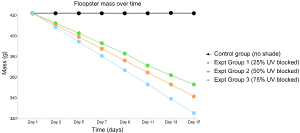
\[ \large{\textbf{IOHOIHEF}} \\ \small \begin{array}{|c|c|c|c|c|c|c|c|c|} \hline \text{Condition} & \text{Day 1} & \text{Day 3} & \text{Day 5} & \text{Day 7} & \text{Day 9} & \text{Day 11} & \text{Day 13} & \text{Day 15} \\ \hline \begin{array}{c}\textbf{Control Group} \\ \text{(no UV blocking)}\end{array} & 421.98 & 422.01 & 422.00 & 421.99 & 421.97 & 421.99 & 422.03 & 421.98 \\ \hline \begin{array}{c}\textbf{Experimental Group 1} \\ \text{(25% UV blocking)}\end{array} & 422.03 & 412.33 & 402.53 & 392.73 & 382.93 & 371.13 & 361.96 & 352.88 \\ \hline \begin{array}{c}\textbf{Experimental Group 2} \\ \text{(50% UV blocking)}\end{array} & 422.07 & 410.53 & 399.03 & 387.53 & 376.03 & 364.53 & 352.88 & 341.38 \\ \hline \begin{array}{c}\textbf{Experimental Group 3} \\ \text{(75% UV blocking)}\end{array} & 422.21 & 408.20 & 394.37 & 380.54 & 366.71 & 352.88 & 339.05 & 325.22 \\ \hline \end{array} \]

An observable is given by \(\boldsymbol{\Omega}.\) We want to find out how it relates to \(\boldsymbol{\Omega}^\dagger.\) Kets and operators have truth independent of any particular representation, but we can calculate inside of a particular basis to simplify our investigations.

In its own basis, we can represent it by \(\boldsymbol{\Omega} = \sum_k \omega_k \ketbra{\omega_k}{\omega_k}.\)

An arbitrary quantum state in this basis is given by \(\ket{\psi} = c_1\ket{\omega_1} + \cdots + c_n\ket{\omega_n}.\)

Operating on the quantum state, we have \(\boldsymbol{\Omega}\ket{\psi} = \sum_k\omega_k\ket{\omega_k}\braket{\omega_k|\psi} = \sum_k\omega_kc_k\ket{\omega_k}.\)

On the other hand \(\bra{\psi}\boldsymbol{\Omega} = \left(c_1^*\bra{\omega_1} + \cdots + c_n^*\bra{\omega_n}\right)\left(\sum_k \omega_k \ketbra{\omega_k}{\omega_k}\right) = \sum_k c_k^*\omega_k\bra{\omega_k} = \sum_k\left(c_k\omega_k^*\ket{\omega_k}\right)^\dagger = \left(\boldsymbol{\Omega}\ket{\psi}\right)^\dagger = \bra{\psi}\boldsymbol{\Omega}^\dagger.\)

Since the quantum state \(\ket{\psi}\) is arbitrary, we have that in general \(\boldsymbol{\Omega} = \boldsymbol{\Omega}^\dagger.\)

\(\SI{1.5}{\electronvolt}\)

\(\SI{4}{\electronvolt}\)

Ideal gas law

The ideal gas law states that the pressure, volume, temperature, and number of molecules in a gas are related by \[\boxed{PV=Nk_BT},\] where \(k_B\) is Boltzmann's constant.

It holds for monatomic gases but requires more serious modification for gases that are diatomic, triatomic, etc. It can be derived from many starting places including the impulse momentum theorem, the partition function, and the absence of correlated motions. It accounts for a number of individual experimental observations that were made prior:

for constant \(T\) and \(N,\) \(P\) and \(V\) are inversely proportional.
for constant \(P\) and \(N,\) \(V\) and \(T\) are directly proportional.
for constant \(V\) and \(N,\) \(P\) and \(T\) are directly proportional.

Taylor expansion

The Taylor series representation of a function is given by

\[f(x) = f(x_0) + f^\prime(x)\rvert_{x = x_0}\left(x - x_0\right) + \frac{1}{2!} f^{\prime\prime}(x)\rvert_{x = x_0}\left(x - x_0\right)^2 + \ldots.\]

which can be found through integration by parts.

Unwieldy analytic expressions can be approximated by expanding into a Taylor series of a small parameter (much less than 1) and keeping the first few terms. For example \(1/\sqrt{1-x} \approx 1 + x/2,\) when \(x \ll 1.\)

The proper time \(\tau\) is given by \(\tau^2 = \left(c\Delta t\right)^2 - \Delta x^2 - \Delta y^2 - \Delta z^2\) and is ensured by the Lorentz transformation to be frame independent. It is equal to the amount of time that passes between two events in their own rest frame, e.g. onboard a spaceship.

\(\tau^2\) classifies spacetime into events that are in the potential future and past or the absolute elsewhere relative to another event. In particular, \(\tau^2\) is zero for trajectories of lightbeams. When \(\tau^2 > 0\) the interval is timelike separated and then \(\tau^2<0\) it is spacelike separate. All causal sequences of events are timelike separated.

The work-energy theorem states that the energy needed to move a particle along a path \(\gamma\) under the force \(\mathbf{F}\) is given by \(W_\gamma = \int_\gamma \mathbf{F}\cdot d\mathbf{x}.\)) Simple manipulations of this result yield expressions for kinetic energy (by making the replacement \(F\rightarrow m\dot{v}\) and evaluating the integral), power (by re-expressing \(dx = dx/dv\cdot dv\) using the chain rule), etc. It is also used in numerical simulations to estimate the free-energy difference between states, e.g. in drug design.

Show me the \(\color{blue}{\textrm{money}}\)

Section One

png:

svg:

png:

svg:

png: svg:

svg:

A cation is a positively charged atom or molecule.

If we strip a neutral \(\ce{Na}\) atom of one electron, is it an anion or a cation?

As the \(\ce{Na}\) atom starts off neutral, it has an equal number of protons and electrons. Stripping off one electron leads to an imbalance of one more proton relative to electrons, so that is it positively charged.

Section 2: Respiration

Respiration procedes according to the following reaction

\[\ce{C6H12O6 + 6O2 -> 6CO2 + 6H2O + energy}.\]

This wiki is incomplete.

\end{array}

+

+

+

5

6

+

7

8

-

Contents