Monte-Carlo Simulation

Monte Carlo simulations define a method of computation that uses a large number of random samples to obtain results. They are often used in physical and mathematical problems and are most useful when it is difficult or impossible to use other mathematical methods. Monte Carlo methods are mainly used in three distinct problem classes: optimization, numerical integration, and generating draws from probability distributions.

Monte Carlo simulations are often used when the problem at hand has a probabilistic component. An expected value of that probabilistic component can be studied using Monte Carlo due to the law of large numbers. With enough data, even though it's sampled randomly, Monte Carlo can hone in on the truth of the problem. For example, we can estimate the value of pi by simply throwing random needles into a circle inscribed within a square that is drawn on the ground. After many needles are dropped, one quadrant of the circle is then examined. The ratio of the number of needles that are inside the square to the number of needles inside the circle is a very good approximation of pi. The more needles that are dropped, the closer the approximation gets.

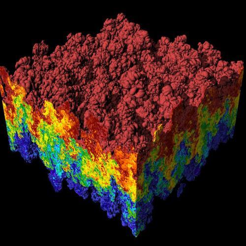
Rayleigh Taylor Instability uses Monte Carlo to predict how two liquids will interact

The most comforting thing about Newtonian mechanics is that everything happens for a reason. For example, if you push one end of the lever, the other end goes up. You throw an object, and it travels in a parabolic path. The physical world is a completely deterministic place: all the future states are derived form the previous ones. For centuries we had this prevailing scientific wisdom, and then came the Copenhagen doctrine, led by Bohr and Heisenberg. The proponents of this doctrine argued that at the most fundamental level, the behavior of a physical system cannot be determined. This led to a serious debate regarding the validity of causal non-determinism, i.e. every event is not caused by previous events. People like Einstein and Schrodinger found this philosophy unacceptable as exemplified by Einstein's often repeated comment: "God does not play dice." The question of causal non-determinism is still unsettled but there is ample evidence to prove that certain systems can only be modeled accurately by stochastic processes. A process is called stochastic if its next step depends on both previous states and some random event.

Most of us are able to calculate the basic probability of occurrence of certain events, but how do we interpret the significance of the results obtained? The answer is that, in this age of fast computers, we can run multiple simulations of an event and record the outcomes and compare the results with the mathematically calculated value! Then in front of our own eyes we can see how powerful the theory of probability is!

The Monte Carlo method is a method of solving problems using statistics. Given the probability that a certain event will occur in certain conditions, a computer can be used to generate those conditions repeatedly.

Monte Carlo method process:

1. Pick a space of possible samples.
2. Randomly sample in that space using a probability distribution.
3. Perform defined operations on the random samples.
4. Aggregate the data.

To tie this process to something more concrete, take the example of estimating pi that is explained in more detail below. The first step in this process is to pick the space of possible samples. That would be the physical space of the circle inscribed within a square. That space is then randomly sampled by throwing needles into it at random. A defined operation of counting the needles is then done. And finally, a ratio is calculated for those needles.

The Monte Carlo process can be a little difficult to accept. If we're just randomly gathering data, how can that help us find a correct answer?

Let's think about a coin. We want to know if the coin is fair or not. A fair coin has these properties

\[P(\text{heads}) = \frac{1}{2} , \quad P(\text{tails}) = \frac{1}{2} . \]

If you flip a coin just one time, what will happen? It will either land on heads or tails. If you flip a coin and it lands on tails, and then you walk away, have you proven that \(P(\text{tails}) = 1\) and that the coin is not fair? Of course not! A fair coin can also land on tails after one try, after all.

Maybe you flip the coin again and it lands on heads, thus proving that \(P(\text{tails}) = P(\text{heads}) = \frac{1}{2}\), and that the coin is fair. But have you actually proven that the coin is fair? Maybe the coin isn't completely fair but it does land on both sides sometimes.

Maybe you flip tails again, and you're even more convinced that \(P(\text{tails}) = 1\). Sadly, we still don't know because both a fair coin and a false coin have the ability to flip tails twice in a row.

The point is that we need to flip this coin a lot before we can be convinced that it's fair. Let's see this with some code. In the following Python snippet, there's a function that takes in the probability that a coin flips a heads (it's o.5 if the coin is fair) and a number of times to flip the coin. It then returns a guess as to the fairness of the coin (again, it's 0.5 if it's fair).

1
2
3
4
5
6
7
8
9

import random

def getCoinProb(headsProb, numFlips):
    prob = 0.0
    for flip in range(numFlips):
        currentFlip = random.random()
        if currentFlip <= headsProb: #Probability of Heads
            prob += 1
    return prob / numFlips

Let's look at a fair coin first. We can flip the coin once, get tails, so the coin looks like it's actually not fair. We then do 5 flips, and it looks better, but we're still not totally convinced that the coin is completely fair. Even after 100 trials, it's close, but not 100%. It takes 100000 flips of the coin for us to start to believe that this coin is fair (and we should do even more to be completely sure).

1
2
3
4
5
6
7
8

>>> getCoinProb(.5, 1)
0.0
>>> getCoinProb(.5, 5)
0.4
>>> getCoinProb(.5, 100)
0.54
>>> getCoinProb(.5, 100000)
0.50065

Now let's flip a false coin. We'll say that this coin flips heads 75% of the time (so it's a really false coin). We flipped it once and actually got tails, way off our expectation! Flipping it 5 times gets us closer to our 75% mark, but it's just as far away from being fair after 5 flips as the actual fair coin. Flipping it 100 and 100000 times gets us closer to our mark.

1
2
3
4
5
6
7
8

>>> getCoinProb(.75, 1)
0.0
>>> getCoinProb(.75, 5)
0.6
>>> getCoinProb(.75, 100)
0.78
>>> getCoinProb(.75, 100000)
0.75006

This is the main point of the Monte Carlo method. When there's something probabilistic (like flipping a coin) that we can't predict, we need to do a lot of trials to make sure we're understanding the system correctly.

One of the most influential figures in the history of probability theory was Blaise Pascal. His interest in the field began when a friend asked him the following question:

"Would it be profitable given 24 rolls of a pair of fair dice to bet against there being at least one double six?"

Write a function that uses Monte Carlo to simulate the probability of getting a pair of 6's within twenty-four rolls of a pair of dice.

---

The probability of rolling a pair of 6's with just one roll is \(\frac{1}{36}\). Therefore the probability of rolling a double six with \(24\) rolls is \(1-\big(\frac{35}{36}\big)^{24}=0.49\).

1 2 3 4 5 6 7 8 9 10 11 12 13 14 15 16

import random def rollDie(): """returns a random int between 1 and 6""" return random.choice([1,2,3,4,5,6]) def Monteprob(numTrials): numwins = 0.0 for i in range(numTrials): for j in range(24): d1 = rollDie() d2 = rollDie() if d1 == 6 and d2 == 6: numwins += 1 break print numwins/numTrials

Now we can test the code to see how the number of trials we make affects the probability outcome.

1 2 3 4 5 6 7 8 9 10 11 12 13 14 15 16 17 18 19 20 21

#100 Trials >>> Monteprob(100) 0.52 >>> Monteprob(100) 0.55 >>> Monteprob(100) 0.54 #10000 Trials >>> Monteprob(10000) 0.4918 >>> Monteprob(10000) 0.4875 >>> Monteprob(10000) 0.4964 #100000 Trials >>> Monteprob(100000) 0.49017 >>> Monteprob(100000) 0.49077 >>> Monteprob(100000) 0.49138

The more trial we do, the closer the answers are to each other. As the number of trials stretches to infinity, we converge on an answer. Here, we can guess from our last set of Monte Carlo runs that the answer is around 0.491 or 49.1%.

Monte Carlo simulation is useful for tackling problems in which nondeterminism plays a role. Interestingly, however, Monte Carlo simulation (and randomized algorithms in general) can be used to solve problems that are not inherently stochastic, i.e., for which there is no uncertainty about outcomes.

Let us imagine a rectangle of height \(h\), width \(b-a\) and area \(A=h(b-a)\) such that the function \(f(x)\) is within the boundaries of the rectangle. Then compute \(n\) pairs of random numbers \(x_{i}\) and \(y_{i}\) with \(a\leq x_{i} \leq b\) and \(0\leq y_{i} \leq h\). The fraction of points \(x_{i}\) and \(y_{i}\) that satisfy the condition \(y_{i}\leq f(x_{i})\) is an estimate of \(f(x)\) to the area of the rectangle. Hence the estimate \(G_{n}\) is given by

\[G_{n}=A\frac{n_{h}}{n},\]

where \(n_{h}\) is the number of hits landed below the curve and \(n\) is the total number of hits on the rectangle.

In numerical integration, methods such as the trapezoidal rule use a deterministic approach. Monte Carlo integration, on the other hand, employs a non-deterministic approach: each realization provides a different outcome. In Monte Carlo, the final outcome is an approximation of the correct value. There is always some error when it comes to approximations, and the approximation of Monte Carlo is only as good as its error bounds. The bounds can be shrunk if more and more samples are collected, though, and that is the power of Monte Carlo.

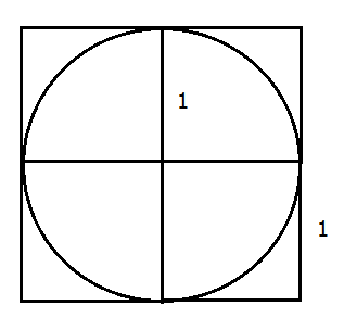
Long before computers were invented, the French mathematicians Buffon (1707-1788) and Laplace (1749-1827) proposed using a stochastic simulation to estimate the value of \(π\). Think about inscribing a circle in a square with sides of length \(2\), so that the radius \(r\) of the circle is of length \(1\).

We have the area of the circle \(\pi r^{2}=\pi\). But what’s \(\pi?\) Buffon suggested that he could estimate the area of a circle by a dropping a large number of needles (which he argued would follow a random path as they fell) in the vicinity of the square. The ratio of the number of needles with tips lying within the square to the number of needles with tips lying within the circle could then be used to estimate the area of the circle:

\[\frac { { A }_{ c } }{ { A }_{ s } } =\frac { \pi { r }^{ 2 } }{ 4{ r }^{ 2 } } \implies \pi =4\frac { { A }_{ c } }{ { A }_{ s } }.\]

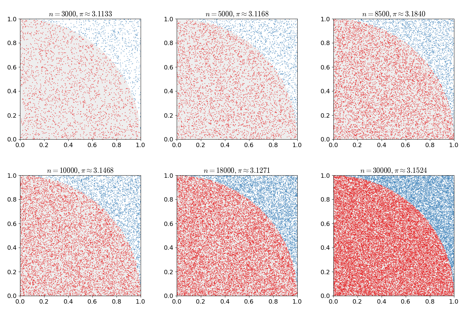
Dropping more and more needles in the circle^[1]

Notice how the more needles we drop in the circle, the closer our approximation gets to the actual value of \(\pi.\)

 1
 2
 3
 4
 5
 6
 7
 8
 9
10
11
12
13
14
15
16
17
18

from random import random
from math import pow, sqrt

trial=1000000
hits = 0
throws = 0
for i in range (1, trial):
    throws += 1
    x = random()
    y = random()
    dist = sqrt(pow(x, 2) + pow(y, 2))
    if dist <= 1.0:
        hits = hits + 1.0

# hits / throws = 1/4 Pi
pi = 4 * (hits / throws)

print("pi is= ",pi)

The above algorithm simulates dropping a needle by first using random to get a pair of positive Cartesian coordinates (\(x\) and \(y\) values). It then uses the Pythagorean theorem to compute the hypotenuse of the right triangle with base \(x\) and height \(y.\) This is the distance of the tip of the needle from the origin (the center of the square). Since the radius of the circle is \(1\), we know that the needle lies within the circle if and only if the distance from the origin is no greater than \(1\). We use this fact to count the number of needles in the circle.

1. Jo, C. Trie. Retrieved June 22, 2016, from https://en.wikipedia.org/wiki/Monte_Carlo_method