Recursive Backtracking

Backtracking can be thought of as a selective tree/graph traversal method. The tree is a way of representing some initial starting position (the parent node) and a final goal state (one of the leaves). Backtracking allows us to deal with situations in which a raw brute-force approach would explode into an impossible number of choices to consider. Backtracking is a sort of refined brute force. At each node, we eliminate choices that are obviously not possible and proceed to recursively check only those that have potential. This way, at each depth of the tree, we mitigate the number of choices to consider in the future.

Suppose you get to a bad leaf. You can backtrack to continue the search for a good leaf by revoking your most recent choice, and trying out the next option in that set of options. If you run out of options, revoke the choice that got you here, and try another choice at that node. If you end up at the root with no options left, there are no good leaves to be found.

Backtracking is essential for solving constraint satisfaction problems, such as crosswords, verbal arithmetic, Sudoku, and many other puzzles. It is also used in solving the knapsack problem, parsing texts and other combinatorial optimization problems.

What’s interesting about backtracking is that we back up only as far as needed to reach a previous decision point with an as-yet-unexplored alternative. In general, that will be at the most recent decision point. Eventually, more and more of these decision points will have been fully explored, and we will have to backtrack further and further. If we backtrack all the way to our initial state and have explored all alternatives from there, we can conclude the particular problem is unsolvable. In such a case, we will have done all the work of the exhaustive recursion and known that there is no viable solution possible.

A permutation of a given set of items is a certain rearrangement of the elements. It can be shown that an array \(A\) of length \(N\) has \(n!\) permutations. For example the array ['J','O','N'] has the following permutations:

1
2
3
4
5
6

['J', 'O', 'N']
['J', 'N', 'O']
['O', 'J', 'N']
['O', 'N', 'J']
['N', 'J', 'O']
['N', 'O', 'J']

The backtracking algorithm applied here is fairly straight forward because the calls are not subject to any constraint. We are not backtracking from an unwanted result, we are merely backtracking to return to a previous state without filtering out unwanted output. This is elaborated a little bit more in the picture and code below:

diag

As shown in the diagram the algorithm is based on swapping. When implemented, the backtracking part is swapping back the items to their previous place after the permutation has been printed.

The following python code shows how this is done:

 1
 2
 3
 4
 5
 6
 7
 8
 9
10
11
12
13

def permutation(list, start, end):
    '''This prints all the permutations of a given list
       it takes the list,the starting and ending indices as input'''
    if (start == end):
        print list
    else:
        for i in range(start, end + 1):
            list[start], list[i] = list[i], list[start]  # The swapping
            permutation(list, start + 1, end)
            list[start], list[i] = list[i], list[start]  # Backtracking


permutation([1, 2, 3], 0, 2)  # The first index of a list is zero

It outputs

1
2
3
4
5
6
7

>>> 
[1, 2, 3]
[1, 3, 2]
[2, 1, 3]
[2, 3, 1]
[3, 2, 1]
[3, 1, 2]

Sudoku is a logic puzzle in which the goal is to fill grid with digits so that each column, each row, and each of the sub-grids that compose the grid contains all of the digits from \(1\) to \(n\).The same single integer may not appear twice in the same row , column or sub-grid.

Let us look at a simplified \(3\times3\) mini version of the original Sudoku puzzle. Here, each cell is a subgrid containing \(1\) element and is trivial distinct. This means we only need to check if the rows and columns contain the integers \(1\),\(2\) and \(3\) with no repetitions.

Below is an example of a mini Sudoku puzzle(left) and its solution (right)

It should be obvious by now that this puzzle is ripe for recursive backtracking. Let us now lay out pseudocode that will help us solve it.

 1
 2
 3
 4
 5
 6
 7
 8
 9
10
11
12
13

function solve( board )
    if the board contains no invalid cells, ie.cells that violate the rules:
        if it is also completely filled out then
            return true
    for each cell in the board
        if the cell is empty
            for each number in {1,2,3}
                replace the current cell with number
                if solve(board) and the board is valid
                    return true
                else
                    backtrack
        return false

The code above is a classic example of backtracking. The function returns true if a given board can be solved. It also solves the given board so the scope of the variable board should be outside the function.

Implement an actual mini \(3\times3\) solver and use it to print the solution\s to the puzzle below

Example solution in python

1 2 3 4 5 6 7 8 9 10 11 12 13 14 15 16 17 18 19 20 21 22 23 24 25 26 27 28 29 30 31 32 33 34 35 36 37 38 39 40 41 42 43 44 45 46 47 48 49 50 51 52 53 54 55 56 57 58 59 60 61 62 63 64

from itertools import * from copy import copy def is_distinct( list ): '''Auxiliary function to is_solved checks if all elements in a list are distinct (ignores 0s though) ''' used = [] for i in list: if i == 0: continue if i in used: return False used.append(i) return True def is_valid( brd ): '''Checks if a 3x3 mini-Sudoku is valid.''' for i in range(3): row = [brd[i][0],brd[i][1],brd[i][2]] if not is_distinct(row): return False col = [brd[0][i],brd[1][i],brd[2][i]] if not is_distinct(col): return False return True def solve( brd , empties = 9): ''' Solves a mini-Sudoku brd is the board empty is the number of empty cells ''' if empties == 0: #Base case return is_valid( brd ) for row,col in product(range(3),repeat=2): #Run through every cell cell = brd[row][col] if cell != 0: #If its not empty jump continue brd2 = copy( brd ) for test in [1,2,3]: brd2[row][col] = test if is_valid(brd2) and solve(brd2,empties-1): return True #BackTrack brd2[row][col] = 0 return False Board = [ [ 0 , 0 , 0 ], [ 1 , 0 , 0 ], [ 0 , 3 , 1 ] ] solve( Board , 9 - 3 ) for row in Board:#Prints a solution print row

It outputs

1 2 3 4

>>> [3, 1, 2] [1, 2, 3] [2, 3, 1]

A more practical and well known example of backtracking is path finding. A robot can for example plan its path in a maze by recurring over the paths and backtracking from the ones that lead no where. This of course requires us to represent the maze in a way that the algorithm is compatible with. A common method is to use a \(2-d\) matrix and values within it to represent obstacles or paths. Below is a simplified version of the maze solving problem that should help clarify the backtracking algorithm.

The Simplified Path Finding Problem

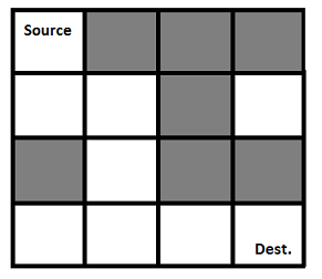
Given an \(N \times N\) matrix of blocks with a source upper left block, we want to find a path from the source to the destination(the lower right block). We can only move downwards and to the left. Also a path is given by \(1\) and a wall is given by \(0\).

The following is an example of of a maze(the black cells are inaccessible)

1
2
3
4

{ 1 , 0 , 0 , 0 }
{ 1 , 1 , 0 , 0 }
{ 0 , 1 , 0 , 0 }
{ 0 , 1 , 1 , 1 }

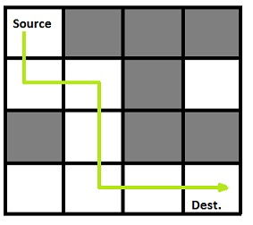
The solution is the follows:

We can now outline a backtracking algorithm that returns an array containing the path in a coordinate form . For example, for the picture above, the solution is \( \large{ (0,0) \rightarrow (1,0) \rightarrow (1,1) \rightarrow (2,1) \rightarrow (3,1) \rightarrow (3,2) \rightarrow (3,3)} \)

1
2
3
4
5
6

If we have reached the destination point
        return an array containing only the position of the destination
else
       a,move in the forwards direction and check if this leads to a solution
       b,if  option a does not work, then move down
      c, if either work, add the current position to the solution obtained at either a or b

An implementation in python looks like the following

 1
 2
 3
 4
 5
 6
 7
 8
 9
10
11
12
13
14
15
16
17
18
19
20
21
22
23
24

def solveMaze( Maze , position , N ):
    # returns a list of the paths taken
    if position == ( N - 1 , N - 1 ):
        return [ ( N - 1 , N - 1 ) ]
    x , y = position
    if x + 1 < N and Maze[x+1][y] == 1:
        a = solveMaze( Maze , ( x + 1 , y ) , N )
        if a != None:
            return [ (x , y ) ] + a

    if y + 1 < N and Maze[x][y+1] == 1:
        b = solveMaze( Maze , (x , y + 1) , N )
        if  b != None:
            return [ ( x , y ) ] + b


Maze = [[ 1 , 0 , 1, 0 , 0],
        [ 1 , 1 , 0, 1 , 0],
        [ 0 , 1 , 0, 1 , 0],
        [ 0 , 1 , 0, 0 , 0],
        [ 1 , 1 , 1, 1 , 1]
        ]

print solveMaze(Maze,(0,0),5)

Contrary to the permutations problem, here we will see an example of backtracking that involves checking a lot of constraints. This does not sound good but having a large number of constraints actually allows us to significantly reduce the search space when we are backtracking. This also means a substantial improvement in run time and performance.

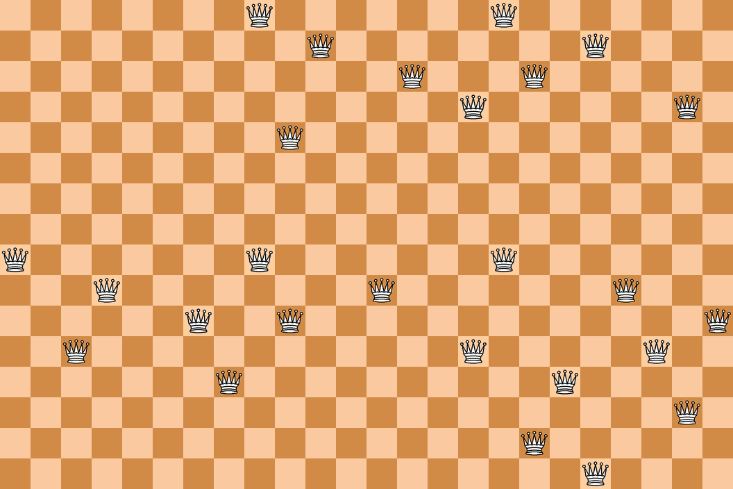
An example of a solution

Image Credit: [wikipedia]

A very common example of backtracking in computer science is the problem of placing \(N\) queens on a checkers board in a way that no two queens attack each other. A checker board consists of \(8 \times 8\) cells. Queens can move vertically, horizontally and diagonally. The problem is computing the number of solutions, not enumerating each individual solution.

 1
 2
 3
 4
 5
 6
 7
 8
 9
10
11
12
13
14
15
16

function solve( board ){
     //Solves the 8queen problem
     if the number of queens on the board equals 8
        return true;
    for position in board.empty_spaces()
        board.placeQueen( position )
        if there are conflicts in the board   
            board.removeQueen(position) //Backtrack
            continue
        else
            if solve(board)
                return true
            else
                return false;
    return false;
}

Because of the nature of chess, when covering the chess board we cut the search space whenever we find a square where we cannot put another queen given our configuration. A backtrack search is most effective here because it eliminates around \(95%\) of the search space. The pseudo-code above shows the specifics of how this can be done.

Ofcourse when actually writing an implementation we worry about data structures and efficient means of actually representing the problem. The python code below shows an example of how an implementation of the backtracking search can be tackled.

8-Queen's problem

---

1 2 3 4 5 6 7 8 9 10 11 12 13 14 15 16 17 18 19 20 21 22 23 24 25 26 27 28 29 30 31 32 33 34 35 36 37 38 39 40 41 42 43 44 45 46 47 48 49 50 51 52 53 54 55 56 57 58 59 60 61 62 63 64 65

from itertools import * import copy class Board: ''' A class to represent the checker board''' def __init__(self , n): #Initializes the class self.board = [ [ None for i in range(8) ] for i in range(8) ] self.pieces = set() def __str__(self): '''Allows us to print the board''' S = '' for i in self.board: S += str(i) + '\n' return S def PlaceQueen(self,row,column): '''Places a queen at row,column''' self.pieces.add( (row , column) ) self.board[row][column] = 'Q' def RemoveQueen(self,row,column): '''Removes a queen from a given 'row' and 'column' ''' self.board[row][column] = None self.pieces.remove( ( row , column ) ) def isAttacking( self, piece1 , piece2 ): '''Checks if piece1 attacks piece2''' if piece1[0] == piece2[0] or piece1[1] == piece2[1]: #Check if they are in same row or col return True '''Time to check if they are attacking diagonally This can be done efficiently via simple algebra The two pices are on the same diagonal if they satisfy an equation of a line containing the two points''' x1 , y1 , x2 , y2 = piece1[1] , piece1[0] ,piece2[1] ,piece2[0] m = float(y2 - y1) / (x2 - x1) if abs(m) != 1.0: return False else: b = y2 - m * x2 return y1 == m * x1 + b def isAttackingAny( self , piece ): '''Checks if piece is being atacked by any other piece in the board''' for piece1 in self.pieces: if self.isAttacking(piece,piece1): return True return False def NQueens( board , n ): if n == 0: return [board] solutions = [] i = 0 for piece1 in product(range(8),repeat=2): if piece1 in board.pieces: continue if not board.isAttackingAny(piece1): i += 1 fresh = copy.deepcopy(board) fresh.PlaceQueen(piece1[0] , piece1[1] ) solutions += NQueens( fresh , n - 1 ) return solutions

8-Queen's problem

---

1 2 3 4 5 6 7 8 9 10 11 12 13 14 15 16 17 18 19 20 21 22 23 24 25 26 27 28 29 30

''' Contributed by: Bipin Oli ''' def isValid(row,pos): if pos>=N or row>=N: return False if pos in sol: return False for i in range(len(sol)): if pos == sol[i]+row-i or pos == sol[i]-(row-i): return False return True def solve(pos,Qc): Qc-=1 sol.append(pos) if Qc==0: return True #Try for i in range(N): if(isValid(N-Qc,i)): if(solve(i,Qc)): return True sol.pop() Qc+=1 return False Queens = int(input().strip()) N=Queens sol=[] for i in range(Queens): if(solve(i,N)): print(sol) sol=[]