Ridge Regression

Tikhonov Regularization, colloquially known as ridge regression, is the most commonly used regression algorithm to approximate an answer for an equation with no unique solution. This type of problem is very common in machine learning tasks, where the "best" solution must be chosen using limited data.

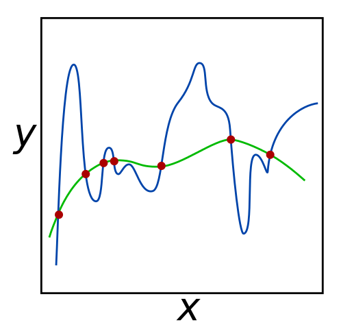
For the given set of red input points, both the green and blue lines minimize error to 0. However, the green line may be more successful at predicting the coordinates of unknown data points, since it seems to generalize the data better. Ridge regression can be used to prefer the green line over the blue line by penalizing large coefficients for \(\boldsymbol{x}\).^[1]

Specifically, for an equation \(\boldsymbol{A}\cdot\boldsymbol{x}=\boldsymbol{b}\) where there is no unique solution for \(\boldsymbol{x}\), ridge regression minimizes \(||\boldsymbol{A}\cdot\boldsymbol{x}-\boldsymbol{b}||^2 + ||\boldsymbol{\Gamma}\cdot\boldsymbol{x}||^2\) to find a solution, where \(\boldsymbol{\Gamma}\) is the user-defined Tikhonov matrix.

Ridge regression is the most commonly used method of regularization for ill-posed problems, which are problems that do not have a unique solution. Simply, regularization introduces additional information to an problem to choose the "best" solution for it.

Suppose the problem at hand is \(\boldsymbol{A}\cdot\textbf{x}=\boldsymbol{b}\), where \(\boldsymbol{A}\) is a known matrix and \(\boldsymbol{b}\) is a known vector. A common approach for determining \(\boldsymbol{x}\) in this situation is ordinary least squares (OLS) regression. This method minimizes the sum of squared residuals: \(||\boldsymbol{A}\cdot\boldsymbol{x} - \boldsymbol{b}||^2\), where \(||\) represents the Euclidean norm, the distance from the origin the resulting vector.

If a unique \(\boldsymbol{x}\) exists, OLS will return the optimal value. However, if multiple solutions exist, OLS may choose any of them. This constitutes an ill-posed problem, where ridge regression is used to prevent overfitting and underfitting. Overfitting occurs when the proposed curve focuses more on noise rather than the actual data, as seen above with the blue line. Conversely, underfitting occurs when the curve does not fit the data well, which can be represented as a line (rather than a curve) that minimizes errors in the image above.

Ridge regression prevents overfitting and underfitting by introducing a penalizing term \(||\boldsymbol{\Gamma} \cdot \boldsymbol{x}||^2\), where \(\boldsymbol{\Gamma}\) represents the Tikhonov matrix, a user defined matrix that allows the algorithm to prefer certain solutions over others. A \(\boldsymbol{\Gamma}\) with large values result in smaller \(\boldsymbol{x}\) values, and can lessen the effects of over-fitting. However, values too large can cause underfitting, which also prevents the algorithm from properly fitting the data. Conversely, small values for \(\boldsymbol{\Gamma}\) result in the same issues as OLS regression, as described in the previous section.

The blue curve minimizes the error of the data points. However, it does not generalize well (it overfits the data). Introducing a \(\boldsymbol{\Gamma}\) term can result in a curve like the black one, which does not minimize errors, but fits the data well.^[2]

A common value for \(\boldsymbol{\Gamma}\) is a multiple of the identity matrix, since this prefers solutions with smaller norms - this is very useful in preventing overfitting. When this is the case (\(\boldsymbol{\Gamma} = \alpha \boldsymbol{I}\), where \(\alpha\) is a constant), the resulting algorithm is a special form of ridge regression called \(L_2\) Regularization.

One commonly used method for determining a proper \(\boldsymbol{\Gamma}\) value is cross validation. Cross validation trains the algorithm on a training dataset, and then runs the trained algorithm on a validation set. \(\boldsymbol{\Gamma}\) values are determined by reducing the percentage of errors of the trained algorithm on the validation set. Overall, choosing a proper value of \(\boldsymbol{\Gamma}\) for ridge regression allows it to properly fit data in machine learning tasks that use ill-posed problems.

Below is some Python code implementing ridge regression.

 1
 2
 3
 4
 5
 6
 7
 8
 9
10
11
12
13
14
15
16
17
18
19
20
21
22
23
24
25
26
27
28
29
30
31
32
33

import numpy as np
import random as rnd

def ridge_regression(A, b, alpha, x):
    # Begin with simple OLS minimization
    ols_term = np.linalg.norm(np.dot(A, x) - b)

    # Add the regularization term
    regularization = np.linarg.norm(alpha * x)

    return ols_term + regularization

def find_best_fit():
    # Create values for A and b
    A = np.matrix(...)
    b = np.matrix(...)

    # Use a moderate value for alpha
    alpha = 3.0

    # Find value of x that minimizes ridge regression error
    min_error = float("inf")
    min_x = np.zeros(...)

    for i in range(1000):
        x = np.random.rand(...)

        error = ridge_regression(A, b, alpha, x)
        if error < min_error:
            min_error = error
            min_x = x

    return min_x

1. Nicoguaro, . Regularization.svg. Retrieved May 31, 2016, from https://en.wikipedia.org/wiki/File:Regularization.svg
2. Ghiles, . Overfitted_Data.svg. Retrieved May 31, 2016, from https://en.wikipedia.org/wiki/File:Overfitted_Data.png