Counting Sort

Counting sort is an efficient algorithm for sorting an array of elements that each have a nonnegative integer key, for example, an array, sometimes called a list, of positive integers could have keys that are just the value of the integer as the key, or a list of words could have keys assigned to them by some scheme mapping the alphabet to integers (to sort in alphabetical order, for instance). Unlike other sorting algorithms, such as mergesort, counting sort is an integer sorting algorithm, not a comparison based algorithm. While any comparison based sorting algorithm requires \(\Omega(n \lg n)\) comparisons, counting sort has a running time of \(\Theta(n)\) when the length of the input list is not much smaller than the largest key value, \(k\), in the list. Counting sort can be used as a subroutine for other, more powerful, sorting algorithms such as radix sort.

An algorithm that maps the following input/output pair is called a sorting algorithm:

Input: An array, \(A\), of size \(n\) of orderable elements. \(A[0,1,...,n-1]\)

Output: A sorted permutation of \(A\), called \(B\), such that \(B[0] \leq B[1] \leq ... \leq B[n-1].\)

Here is what it means for an array to be sorted.

An array \(A\) is sorted if and only if for all \(i<j\), \(A[i] \leq A[j].\ _\square\)

By convention, empty arrays and singleton arrays (arrays consisting of only one element) are always sorted. This is a key point for the base case of many sorting algorithms.

Counting sort assumes that each of the \(n\) input elements in a list has a key value ranging from \(0\) to \(k\), for some integer \(k\). For each element in the list, counting sort determines the number of elements that are less than it. Counting sort can use this information to place the element directly into the correct slot of the output array.

Counting sort uses three lists: the input list, \(A[0,1, \dots, n]\), the output list, \(B[0,1, \dots, n]\), and a list that serves as temporary memory, \(C[0,1, \dots, k]\). Note that \(A\) and \(B\) have \(n\) slots (a slot for each element), while \(C\) contains \(k\) slots (a slot for each key value).

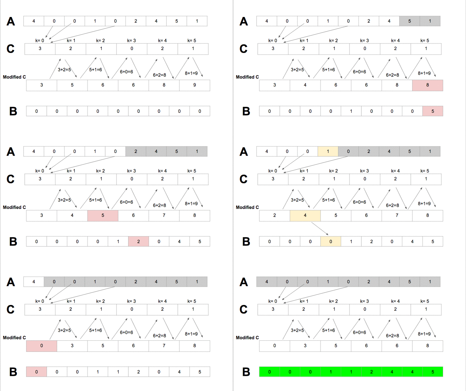
Counting sort starts by going through \(A\), and for each element \(A[i]\), it goes to the index of \(C\) that has the same value as \(A[i]\) (so it goes to \(C[A[i]]\)) and increments the value of \(C[A[i]]\) by one. This means that if \(A\) has seven \(0\)’s in its list, after counting sort has gone through all \(n\) elements of \(A\), the value at \(C[0]\) will be \(7\). Similarly, if \(A\) has two \(4\)’s, after counting sort has gone through all of the elements of \(A\), \(C[4]\) (using 0 indexing) will be equal to \(2\). In this step, \(C\) keeps track of how many elements in \(A\) there are that have the same value of a particular index in \(C\). In other words, the indices of \(C\) correspond to the values of elements in \(A\), and the values in \(C\) correspond to the total number of times that a value in \(A\) appears in \(A\).

Next, modify \(C\) so that each \(C[i]\) includes the number of elements less than or equal to it. This can be accomplished by going through \(C\) and replacing each \(C[i]\) value with \(C[i] + C[i-1]\). This step allows counting sort to determine at what index in \(B\) an element should be placed.

Then, starting at the end of \(A\), add elements to \(B\) by checking the value of \(A[i]\), going to \(C[A[i]]\), writing the value of the element at \(A[i]\) to \(B[C[A[i]]]\). Finally, decrement the value of \(C[A[i]]\) by \(1\) since that slot in \(B\) is now occupied.

This animation illustrates counting sort:

Here is one way to implement counting sort in Python:

 1
 2
 3
 4
 5
 6
 7
 8
 9
10
11
12
13
14
15
16
17
18
19
20
21
22
23
24
25
26

def counting_sort(A, digit, radix):
    #"A" is a list to be sorted, radix is the base of the number system, digit is the digit
    #we want to sort by

    #create a list B which will be the sorted list
    B = [0]*len(A)
    C = [0]*int(radix)
    #counts the number of occurences of each digit in A 
    for i in range(0, len(A)):
        digit_of_Ai = (A[i]/radix**digit)%radix
        C[digit_of_Ai] = C[digit_of_Ai] +1 
        #now C[i] is the value of the number of elements in A equal to i

    #this FOR loop changes C to show the cumulative # of digits up to that index of C
    for j in range(1,radix):
        C[j] = C[j] + C[j-1]
        #here C is modifed to have the number of elements <= i
    for m in range(len(A)-1, -1, -1): #to count down (go through A backwards)
        digit_of_Ai = (A[m]/radix**digit)%radix
        C[digit_of_Ai] = C[digit_of_Ai] -1
        B[C[digit_of_Ai]] = A[m]

    return B

#alist = [9,3,1,4,5,7,7,2,2]
#print counting_sort(alist,0,10)

Counting sort has a \(O(k+n)\) running time.

The first loop goes through \(A\), which has \(n\) elements. This step has a \(O(n)\) running time. The second loop iterates over \(k\), so this step has a running time of \(O(k)\). The third loop iterates through \(A\), so again, this has a running time of \(O(n)\). Therefore, the counting sort algorithm has a running time of \(O(k+n)\).

Counting sort is efficient if the range of input data, \(k\), is not significantly greater than the number of objects to be sorted, \(n\).

Counting sort is a stable sort with a space complexity of \(O(k + n)\).