Log-normal Distribution
The log-normal distribution is the probability distribution of a random variable whose logarithm follows a normal distribution. It models phenomena whose relative growth rate is independent of size, which is true of most natural phenomena including the size of tissue and blood pressure, income distribution, and even the length of chess games.
Contents
Formal Definition
Let \(Z\) be a standard normal variable, which means the probability distribution of \(Z\) is normal centered at 0 and with variance 1. Then a log-normal distribution is defined as the probability distribution of a random variable
\[X = e^{\mu+\sigma Z},\]
where \(\mu\) and \(\sigma\) are the mean and standard deviation of the logarithm of \(X\), respectively.
The term "log-normal" comes from the result of taking the logarithm of both sides:
\[\log X = \mu +\sigma Z.\]
As \(Z\) is normal, \(\mu+\sigma Z\) is also normal (the transformations just scale the distribution, and do not affect normality), meaning that the logarithm of \(X\) is normally distributed (hence the term log-normal).
Finding the Log-normal Distribution
The log-normal distribution satisfies
\[f_X(x) = \frac{1}{\sigma x\sqrt{2\pi}}e^{-\dfrac{(\ln x-\mu)^2}{2\sigma^2}},\]
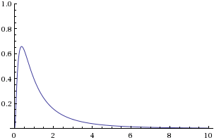
which is a consequence of the change of variable theorem and a small amount of calculus. Unfortunately, this form is very difficult to work with by hand, so it is generally more useful to consider the key properties of the distribution (e.g. the mean and tendencies). For this reason, it is worth examining the result when \(\mu=0, \sigma=1\) (i.e. standard conditions):

Note that the distribution is skewed to the right, and the mode is roughly .35 (in fact, it is \(\frac{1}{e}\), as the next section shows). This, along with the general shape of the curve, is generally sufficient information to draw a reasonably accurate approximation of the graph.
Properties of the Log-normal Distribution
There are several important values that give information about a particular probability distribution. The most important are as follows:
- The mean, or expected value, of a distribution gives useful information about what average one would expect from a large number of repeated trials.
- The median of a distribution is another measure of central tendency, useful when the distribution contains outliers (i.e. particularly large/small values) that make the mean misleading.
- The mode of a distribution is the value that has the highest probability of occurring.
- The variance of a distribution measures how "spread out" the data is. Related is the standard deviation, the square root of the variance, useful due to being in the same units as the data.
These values are often easier to calculate for a continuous probability distribution (such as the log-normal one), but as their calculation involves a fair amount of calculus, the explanation will be brief.
The mean of the log-normal distribution is \[m = e^{\mu+\frac{\sigma^2}{2}},\] which also means that \(\mu\) can be calculated from \(m\): \[\mu = \ln m - \frac{1}{2}\sigma^2.\] These both derive from the mean of the normal distribution.
\[\]
The median of the log-normal distribution is \[\text{Med}[X] = e^{\mu},\] which is derived by setting the cumulative distribution equal to 0.5 and solving the resulting equation.
\[\]
The mode of the log-normal distribution is \[\text{Mode}[X] = e^{\mu-\sigma^2},\] which is derived by setting the derivative of the p.d.f. in the previous section to 0, as the mode represents the global maximum of the distribution.
\[\]
Finally, the variance of the log-normal distribution is \[\text{Var}[X] = (e^{\sigma^2}-1)e^{2\mu+\sigma^2},\] which can also be written as \(\big(e^{\sigma^2}-1\big)m^2\), where \(m\) is the mean of the distribution above.
Practical Applications
For most natural growth processes, the growth rate is independent of size, so the log-normal distribution is followed. As a result, the log-normal distribution has heavy applications to biology and finance, two areas where growth is an important area of study. In particular, epidemics and stock prices tend to follow a log-normal distribution. Other applications include technological ones, such as the file size of publicly available files and time to repair a maintainable system, engineering considerations such as the sizes of cities, and physical ones such as friction coefficients.
The distribution also occurs in seemingly unlikely areas, most notably in the number of moves a chess game takes to end. Based on games played on FICS (Free Internet Chess Server), the number of half-moves is shown in the below image[1]:

which is approximated very well by a log-normal curve.
References
[1] Stackexchange. What is the average length of a game of chess?. Retrieved March 2nd, 2016 from http://chess.stackexchange.com/a/4899